Algorithmic trading in less than 100 lines of Python code

Algorithmic Trading

Algorithmic trading refers to the computerized, automated trading of financial instruments (based on some algorithm or rule) with little or no human intervention during trading hours. Almost any kind of financial instrument — be it stocks, currencies, commodities, credit products or volatility — can be traded in such a fashion. Not only that, in certain market segments, algorithms are responsible for the lion’s share of the trading volume. The books The Quants by Scott Patterson and More Money Than God by Sebastian Mallaby paint a vivid picture of the beginnings of algorithmic trading and the personalities behind its rise.

The barriers to entry for algorithmic trading have never been lower. Not too long ago, only institutional investors with IT budgets in the millions of dollars could take part, but today even individuals equipped only with a notebook and an Internet connection can get started within minutes. A few major trends are behind this development:

• Open source software: Every piece of software that a trader needs to get started in algorithmic trading is available in the form of open source; specifically, Python has become the language and ecosystem of choice.
• Open data sources: More and more valuable data sets are available from open and free sources, providing a wealth of options to test trading hypotheses and strategies.
• Online trading platforms: There is a large number of online trading platforms that provide easy, standardized access to historical data (via RESTful APIs) and real-time data (via socket streaming APIs), and also offer trading and portfolio features (via programmatic APIs).

This article shows you how to implement a complete algorithmic trading project, from backtesting the strategy to performing automated, real-time trading. Here are the major elements of the project:

• Strategy: I chose a time series momentum strategy (cf. Moskowitz, Tobias, Yao Hua Ooi, and Lasse Heje Pedersen (2012): “Time Series Momentum.” Journal of Financial Economics, Vol. 104, 228-250.), which basically assumes that a financial instrument that has performed well/badly will continue to do so.
• Platform: I chose Oanda; it allows you to trade a variety of leveraged contracts for differences (CFDs), which essentially allow for directional bets on a diverse set of financial instruments (e.g. currencies, stock indices, commodities).
• Data: We’ll get all our historical data and streaming data from Oanda.
• Software: We’ll use Python in combination with the powerful data analysis library pandas, plus a few additional Python packages.

The following assumes that you have a Python 3.5 installation available with the major data analytics libraries, like NumPy and pandas, included. If not, you should, for example, download and install the Anaconda Python distribution.

Oanda Account

At http://oanda.com, anyone can register for a free demo (“paper trading”) account within minutes. Once you have done that, to access the Oanda API programmatically, you need to install the relevant Python package:

pip install oandapy

To work with the package, you need to create a configuration file with filename oanda.cfg that has the following content:

[oanda]
account_id = YOUR_ACCOUNT_ID
access_token = YOU_ACCESS_TOKEN

Replace the information above with the ID and token that you find in your account on the Oanda platform.

In [1]:
import configparser  # 1 
import oandapy as opy  # 2

config = configparser.ConfigParser()  # 3
config.read('oanda.cfg')  # 4

oanda = opy.API(environment='practice',
                access_token=config['oanda']['access_token'])  # 5

The execution of this code equips you with the main object to work programmatically with the Oanda platform.

Backtesting

We have already set up everything needed to get started with the backtesting of the momentum strategy. In particular, we are able to retrieve historical data from Oanda. The instrument we use is EUR_USD and is based on the EUR/USD exchange rate.

The first step in backtesting is to retrieve the data and to convert it to a pandas DataFrame object. The data set itself is for the two days December 8 and 9, 2016, and has a granularity of one minute. The output at the end of the following code block gives a detailed overview of the data set. It is used to implement the backtesting of the trading strategy.

In [2]:
import pandas as pd  # 6

data = oanda.get_history(instrument='EUR_USD',  # our instrument
                         start='2016-12-08',  # start data
                         end='2016-12-10',  # end date
                         granularity='M1')  # minute bars  # 7

df = pd.DataFrame(data['candles']).set_index('time')  # 8

df.index = pd.DatetimeIndex(df.index)  # 9

df.info() # 10

<class 'pandas.core.frame.DataFrame'>
DatetimeIndex: 2658 entries, 2016-12-08 00:00:00 to 2016-12-09 21:59:00
Data columns (total 10 columns):
closeAsk    2658 non-null float64
closeBid    2658 non-null float64
complete    2658 non-null bool
highAsk     2658 non-null float64
highBid     2658 non-null float64
lowAsk      2658 non-null float64
lowBid      2658 non-null float64
openAsk     2658 non-null float64
openBid     2658 non-null float64
volume      2658 non-null int64
dtypes: bool(1), float64(8), int64(1)
memory usage: 210.3 KB

Second, we formalize the momentum strategy by telling Python to take the mean log return over the last 15, 30, 60, and 120 minute bars to derive the position in the instrument. For example, the mean log return for the last 15 minute bars gives the average value of the last 15 return observations. If this value is positive, we go/stay long the traded instrument; if it is negative we go/stay short. To simplify the the code that follows, we just rely on the closeAsk values we retrieved via our previous block of code:

In [3]:
import numpy as np  # 11

df['returns'] = np.log(df['closeAsk'] / df['closeAsk'].shift(1))  # 12

cols = []  # 13

for momentum in [15, 30, 60, 120]:  # 14
    col = 'position_%s' % momentum  # 15
    df[col] = np.sign(df['returns'].rolling(momentum).mean())  # 16
    cols.append(col)  # 17

Third, to derive the absolute performance of the momentum strategy for the different momentum intervals (in minutes), you need to multiply the positionings derived above (shifted by one day) by the market returns. Here’s how to do that:

In [4]:
%matplotlib inline
import seaborn as sns; sns.set()  # 18

strats = ['returns']  # 19

for col in cols:  # 20
    strat = 'strategy_%s' % col.split('_')[1]  # 21
    df[strat] = df[col].shift(1) * df['returns']  # 22
    strats.append(strat)  # 23

df[strats].dropna().cumsum().apply(np.exp).plot()  # 24

Out[4]:
<matplotlib.axes._subplots.AxesSubplot at 0x11a9c6a20>

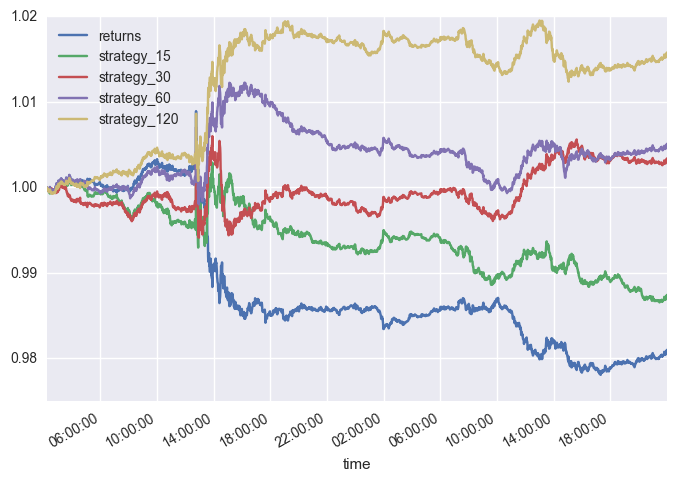
Inspection of the plot above reveals that, over the period of the data set, the traded instrument itself has a negative performance of about -2%. Among the momentum strategies, the one based on 120 minutes performs best with a positive return of about 1.5% (ignoring the bid/ask spread). In principle, this strategy shows “real alpha“: it generates a positive return even when the instrument itself shows a negative one.

Automated Trading

Once you have decided on which trading strategy to implement, you are ready to automate the trading operation. To speed up things, I am implementing the automated trading based on twelve five-second bars for the time series momentum strategy instead of one-minute bars as used for backtesting. A single, rather concise class does the trick:

In [5]:
class MomentumTrader(opy.Streamer):  # 25
    def __init__(self, momentum, *args, **kwargs):  # 26
        opy.Streamer.__init__(self, *args, **kwargs)  # 27
        self.ticks = 0  # 28
        self.position = 0  # 29
        self.df = pd.DataFrame()  # 30
        self.momentum = momentum  # 31
        self.units = 100000  # 32
    def create_order(self, side, units):  # 33
        order = oanda.create_order(config['oanda']['account_id'], 
            instrument='EUR_USD', units=units, side=side,
            type='market')  # 34
        print('\n', order)  # 35
    def on_success(self, data):  # 36
        self.ticks += 1  # 37
        # print(self.ticks, end=', ')
        # appends the new tick data to the DataFrame object
        self.df = self.df.append(pd.DataFrame(data['tick'],
                                 index=[data['tick']['time']]))  # 38
        # transforms the time information to a DatetimeIndex object
        self.df.index = pd.DatetimeIndex(self.df['time'])  # 39
        # resamples the data set to a new, homogeneous interval
        dfr = self.df.resample('5s').last()  # 40
        # calculates the log returns
        dfr['returns'] = np.log(dfr['ask'] / dfr['ask'].shift(1))  # 41
        # derives the positioning according to the momentum strategy
        dfr['position'] = np.sign(dfr['returns'].rolling( 
                                      self.momentum).mean())  # 42
        if dfr['position'].ix[-1] == 1:  # 43
            # go long
            if self.position == 0:  # 44
                self.create_order('buy', self.units)  # 45
            elif self.position == -1:  # 46
                self.create_order('buy', self.units * 2)  # 47
            self.position = 1  # 48
        elif dfr['position'].ix[-1] == -1:  # 49
            # go short
            if self.position == 0:  # 50
                self.create_order('sell', self.units)  # 51
            elif self.position == 1: # 52
                self.create_order('sell', self.units * 2)  # 53
            self.position = -1  # 54
        if self.ticks == 250:  # 55
            # close out the position
            if self.position == 1:  # 56
                self.create_order('sell', self.units)  # 57
            elif self.position == -1:  # 58
                self.create_order('buy', self.units)  # 59
            self.disconnect()  # 60

The code below lets the MomentumTrader class do its work. The automated trading takes place on the momentum calculated over 12 intervals of length five seconds. The class automatically stops trading after 250 ticks of data received. This is arbitrary but allows for a quick demonstration of the MomentumTrader class.

In [6]:
mt = MomentumTrader(momentum=12, environment='practice',
                    access_token=config['oanda']['access_token'])
mt.rates(account_id=config['oanda']['account_id'],
         instruments=['DE30_EUR'], ignore_heartbeat=True)

{'price': 1.04858, 'time': '2016-12-15T10:29:31.000000Z', 'tradeReduced': {}, 'tradesClosed': [], 'tradeOpened': {'takeProfit': 0, 'id': 10564874832, 'trailingStop': 0, 'side': 'buy', 'stopLoss': 0, 'units': 100000}, 'instrument': 'EUR_USD'}

 {'price': 1.04805, 'time': '2016-12-15T10:29:46.000000Z', 'tradeReduced': {}, 'tradesClosed': [{'side': 'buy', 'id': 10564874832, 'units': 100000}], 'tradeOpened': {'takeProfit': 0, 'id': 10564875194, 'trailingStop': 0, 'side': 'sell', 'stopLoss': 0, 'units': 100000}, 'instrument': 'EUR_USD'}

 {'price': 1.04827, 'time': '2016-12-15T10:29:46.000000Z', 'tradeReduced': {}, 'tradesClosed': [{'side': 'sell', 'id': 10564875194, 'units': 100000}], 'tradeOpened': {'takeProfit': 0, 'id': 10564875229, 'trailingStop': 0, 'side': 'buy', 'stopLoss': 0, 'units': 100000}, 'instrument': 'EUR_USD'}

 {'price': 1.04806, 'time': '2016-12-15T10:30:08.000000Z', 'tradeReduced': {}, 'tradesClosed': [{'side': 'buy', 'id': 10564875229, 'units': 100000}], 'tradeOpened': {'takeProfit': 0, 'id': 10564876308, 'trailingStop': 0, 'side': 'sell', 'stopLoss': 0, 'units': 100000}, 'instrument': 'EUR_USD'}

 {'price': 1.04823, 'time': '2016-12-15T10:30:10.000000Z', 'tradeReduced': {}, 'tradesClosed': [{'side': 'sell', 'id': 10564876308, 'units': 100000}], 'tradeOpened': {'takeProfit': 0, 'id': 10564876466, 'trailingStop': 0, 'side': 'buy', 'stopLoss': 0, 'units': 100000}, 'instrument': 'EUR_USD'}

 {'price': 1.04809, 'time': '2016-12-15T10:32:27.000000Z', 'tradeReduced': {}, 'tradesClosed': [{'side': 'buy', 'id': 10564876466, 'units': 100000}], 'tradeOpened': {}, 'instrument': 'EUR_USD'}

The output above shows the single trades as executed by the MomentumTrader class during a demonstration run. The screenshot below shows the fxTradePractice desktop application of Oanda where a trade from the execution of the MomentumTrader class in EUR_USD is active.

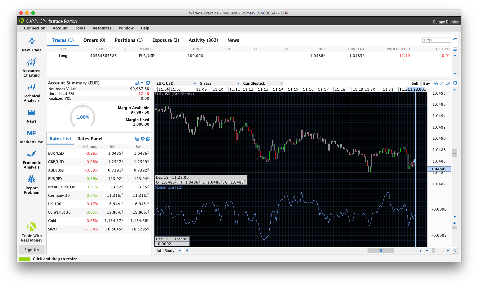
All example outputs shown in this article are based on a demo account (where only paper money is used instead of real money) to simulate algorithmic trading. To move to a live trading operation with real money, you simply need to set up a real account with Oanda, provide real funds, and adjust the environment and account parameters used in the code. The code itself does not need to be changed.

Conclusions

This article shows that you can start a basic algorithmic trading operation with fewer than 100 lines of Python code. In principle, all the steps of such a project are illustrated, like retrieving data for backtesting purposes, backtesting a momentum strategy, and automating the trading based on a momentum strategy specification. The code presented provides a starting point to explore many different directions: using alternative algorithmic trading strategies, trading alternative instruments, trading multiple instruments at once, etc.

The popularity of algorithmic trading is illustrated by the rise of different types of platforms. For example, Quantopian — a web-based and Python-powered backtesting platform for algorithmic trading strategies — reported at the end of 2016 that it had attracted a user base of more than 100,000 people. Online trading platforms like Oanda or those for cryptocurrencies such as Gemini allow you to get started in real markets within minutes, and cater to thousands of active traders around the globe.