Capturing semantic meanings using deep learning

Word embedding is a technique that treats words as vectors whose relative similarities correlate with semantic similarity. This technique is one of the most successful applications of unsupervised learning. Natural language processing (NLP) systems traditionally encode words as strings, which are arbitrary and provide no useful information to the system regarding the relationships that may exist between different words. Word embedding is an alternative technique in NLP, whereby words or phrases from the vocabulary are mapped to vectors of real numbers in a low-dimensional space relative to the vocabulary size, and the similarities between the vectors correlate with the words’ semantic similarity.

For example, let’s take the words woman, man, queen, and king. We can get their vector representations and use basic algebraic operations to find semantic similarities. Measuring similarity between vectors is possible using measures such as cosine similarity. So, when we subtract the vector of the word man from the vector of the word woman, then its cosine distance would be close to the distance between the word queen minus the word king (see Figure 1).

W("woman")−W("man") ≃ W("queen")−W("king")

Many different types of models were proposed for representing words as continuous vectors, including latent semantic analysis (LSA) and latent Dirichlet allocation (LDA). The idea behind those methods is that words that are related will often appear in the same documents. For instance, backpack, school, notebook, and teacher are probably likely to appear together. But school, tiger, apple, and basketball would probably not appear together consistently. To represent words as vectors — using the assumption that similar words will occur in similar documents — LSA creates a matrix, whereby the rows represent unique words and the columns represent each paragraph. Then, LSA applies singular value decomposition (SVD), which is used to reduce the number of rows while preserving the similarity structure among columns.The problem is that those models become computationally very expensive on large data.

Instead of computing and storing large amounts of data, we can try to create a neural network model that will be able to learn the relationship between the words and do it efficiently.

Word2Vec

The most popular word embedding model is word2vec, created by Mikolov, et al., in 2013. The model showed great results and improvements in efficiency. Mikolov, et al., presented the negative-sampling approach as a more efficient way of deriving word embeddings. You can read more about it here.

The model can use either of two architectures to produce a distributed representation of words: continuous bag-of-words (CBOW) or continuous skip-gram.

We’ll look at both of these architectures next.

The CBOW model

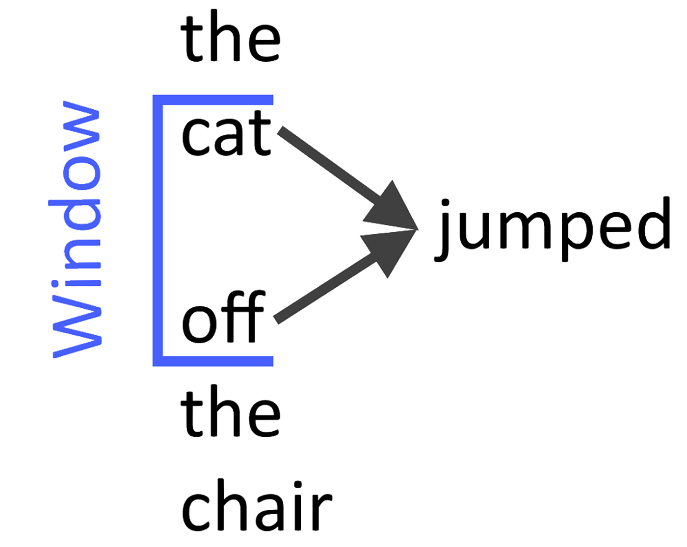
In the CBOW architecture, the model predicts the current word from a window of surrounding context words. Mikolov, et al., thus use both the n words before and after the target word w to predict it.

A sequence of words is equivalent to a set of items. Therefore, it is also possible to replace the terms word and item, which allows for applying the same method for collaborative filtering and recommender systems. CBOW is several times faster to train than the skip-gram model and has slightly better accuracy for the words that appear frequently (see Figure 2).

The continuous skip-gram model

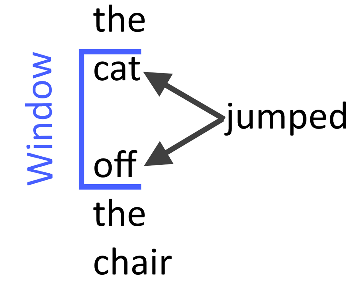
In the skip-gram model, instead of using the surrounding words to predict the center word, it uses the center word to predict the surrounding words (see Figure 3). According to Mikolov, et al., skip-gram works well with a small amount of the training data and does a good job of representing even rare words and phrases.

Coding

(You can find the code for the following example at GitHub repo.)

The great thing about this model is that it works well for many languages.

All we have to do is download a big data set for the language that we need.

Looking to Wikipedia for a big data set

We can look to Wikipedia for any given language. To obtain a big data set, follow these steps:

• Find the ISO 639 code for your desired language: List of ISO 639 codes
• Go to: https://dumps.wikimedia.org/wiki/latest/
• Download wiki-latest-pages-articles.xml.bz2

Next, to make things easy, we will install gensim, a Python package that implements word2vec.

pip install --upgrade gensim

We need to create the corpus from Wikipedia, which we will use to train the word2vec model. The output of the following code is “wiki..text”—which contains all the words of all the articles in Wikipedia, segregated by language.

from gensim.corpora import WikiCorpus

language_code = "he"
inp = language_code+"wiki-latest-pages-articles.xml.bz2"
outp = "wiki.{}.text".format(language_code)
i = 0

print("Starting to create wiki corpus")
output = open(outp, 'w')
space = " "
wiki = WikiCorpus(inp, lemmatize=False, dictionary={})
for text in wiki.get_texts():
  article = space.join([t.decode("utf-8") for t in text])

  output.write(article + "\n")
  i = i + 1
  if (i % 1000 == 0):
    print("Saved " + str(i) + " articles")

output.close()
print("Finished - Saved " + str(i) + " articles")

Training the model

The parameters are as follows:

• size: the dimensionality of the vectors
  • bigger size values require more training data, but can lead to more accurate models
• window: the maximum distance between the current and predicted word within a sentence
• min_count: ignore all words with total frequency lower than this

import multiprocessing
from gensim.models import Word2Vec
from gensim.models.word2vec import LineSentence

language_code = "he"
inp = "wiki.{}.text".format(language_code)
out_model = "wiki.{}.word2vec.model".format(language_code)
size = 100
window = 5
min_count = 5

start = time.time()

model = Word2Vec(LineSentence(inp), sg = 0, # 0=CBOW , 1= SkipGram
       size=size, window=window, min_count=min_count, workers=multiprocessing.cpu_count())

# trim unneeded model memory = use (much) less RAM
model.init_sims(replace=True)

print(time.time()-start)

model.save(out_model)

Training word2vec took 18 minutes.

fastText

Facebook’s Artificial Intelligence Research (FAIR) lab recently released fastText, a library that is based on the work reported in the paper “Enriching Word Vectors with Subword Information,” by Bojanowski, et al. fastText is different from word2vec in that each word is represented as a bag-of-character n-grams. A vector representation is associated with each character n-gram, and words are represented as the sum of these representations.

Using Facebook’s new library is easy:

pip install fasttext

Training the model:

start = time.time()

language_code = "he"
inp = "wiki.{}.text".format(language_code)
output = "wiki.{}.fasttext.model".format(language_code)
model = fasttext.cbow(inp,output)

print(time.time()-start)

Training fastText’s model took 13 minutes.

Evaluating embeddings: Analogies

Next, let’s evaluate the models by testing them on our previous example:

W(“woman”) ≃ W(“man”)+ W(“queen”)− W(“king”)

The following code first computes the weighted average of the positive and negative words.

After that, it calculates the dot product between the vector representation of all the test words and the weighted average.

In our case, the test words are the entire vocabulary. At the end, we print the word that had the highest cosine similarity with the weighted average of the positive and negative words.

import numpy as np
from gensim.matutils import unitvec

def test(model,positive,negative,test_words):

  mean = []
  for pos_word in positive:
    mean.append(1.0 * np.array(model[pos_word]))

  for neg_word in negative:
    mean.append(-1.0 * np.array(model[neg_word]))

  # compute the weighted average of all words
  mean = unitvec(np.array(mean).mean(axis=0))

  scores = {}
  for word in test_words:

    if word not in positive + negative:

      test_word = unitvec(np.array(model[word]))

      # Cosine Similarity
      scores[word] = np.dot(test_word, mean)

  print(sorted(scores, key=scores.get, reverse=True)[:1])

Next, we want to test our original example.

Testing it on fastText and gensim’s word2vec:

positive_words = ["queen","man"]

negative_words = ["king"]

# Test Word2vec
print("Testing Word2vec")
model = word2vec.getModel()
test(model,positive_words,negative_words,model.vocab)

# Test Fasttext
print("Testing Fasttext")
model = fasttxt.getModel()
test(model,positive_words,negative_words,model.words)

Results

Testing Word2vec
  [‘woman’]
Testing Fasttext
  [‘woman’]

These results mean that the process works both on fastText and gensim’s word2vec!

W("woman") ≃ W("man")+ W("queen")− W("king")

And as you can see, the vectors actually capture the semantic relationship between the words.

The ideas presented by the models that we described can be used for many different applications, allowing businesses to predict the next applications they will need, perform sentiment analysis, represent biological sequences, perform semantic image searches, and more.