 Cubes. (source: Michael Pardo on Flickr)
 Uber’s mission is to provide “transportation as reliable as running water, everywhere, for everyone.” To fulfill this promise, Uber relies on making data-driven decisions at every level, and most of these decisions can benefit from faster data processing. For example, using data to understand areas for growth or accessing of fresh data by the city operations team to debug each city. Needless to say, the choice of data processing systems and the necessary SLAs are the topics of daily conversations between the data team and the users at Uber.
In this post, I would like to discuss the choices of data processing systems for near-real-time use cases, based on experiences building data infrastructure at Uber as well as drawing from previous experiences. In this post, I argue that by adding new incremental processing primitives to existing Hadoop technologies, we will be able to solve a lot more problems, at reduced cost, and in a unified manner. At Uber, we are building our systems to tackle the problems outlined here and are open to collaborating with like-minded organizations interested in this space.
Near-real-time use cases
First, let’s establish the kinds of use cases we are talking about: cases in which up to one-hour latency is tolerable are well understood and mostly can be executed using traditional batch processing via MapReduce/Spark, coupled with incremental ingestion of data into Hadoop/S3. On the other extreme, cases needing less than one to two seconds of latency typically involve pumping your data into a scale-out key value store (having worked on one at scale) and querying that. Stream processing systems like Storm, Spark Streaming, and Flink have carved out a niche of operating really well at practical latencies of around one to five minutes, and are needed for things like fraud detection, anomaly detection, or system monitoring—basically, those decisions made by machines with quick turnaround or humans staring at computer screens as their day job.
That leaves us with a wide chasm of five-minute to one-hour end-to-end processing latency, which I refer to in this post as near-real-time. Most such cases are either powering business dashboards and/or aiding some human decision-making. Here are some examples where near-real-time could be applicable:
- Observing whether something was anomalous across the board in the last x minutes;
- Gauging how well the experiments running on the website performed in the last x minutes;
- Rolling up business metrics at x-minute intervals
- Extracting features for a machine-learning pipeline in the last x minutes.

Incremental processing via “mini” batches
The choices to tackle near-real-time use cases are pretty open ended. Stream processing can provide low latency, with budding SQL capabilities, but it requires the queries to be predefined to work well. Proprietary warehouses have a lot of features (e.g., transactions, indexes) and can support ad hoc and predefined queries, but such proprietary warehouses are typically limited in scale and are expensive. Batch processing can tackle massive scale and provides mature SQL support via Spark SQL/Hive, but the processing styles typically involve larger latency. With such fragmentation, users often end up making their choices based on available hardware and operational support within their organizations. We will circle back to these challenges at the conclusion of this post.
For now, I’d like to outline some technical benefits to tackling near-real-time use cases via “mini” batch jobs run every x minutes, using Spark/MR as opposed to running stream-processing jobs. Analogous to “micro” batches in Spark Streaming (operating at second-by-second granularity), “mini” batches operate at minute-by-minute granularity. Throughout the post, I use the term “incremental processing” collectively to refer to this style of processing.
Increased efficiency
Incrementally processing new data in “mini” batches could be a much more efficient use of resources for the organization. Let’s take a concrete example, where we have a stream of Kafka events coming in at 10K/sec and we want to count the number of messages in the last 15 minutes across some dimensions. Most stream-processing pipelines use an external result store (e.g., Cassandra, ElasticSearch) to keep aggregating the count, and keep the YARN/Mesos containers running the whole time. This makes sense in the less-than-five-minute latency windows such pipelines operate on. In practice, typical YARN container start-up costs tend to be around a minute. In addition, to scale the writes to the result stores, we often end up buffering and batching updates, and this protocol needs the containers to be long running.
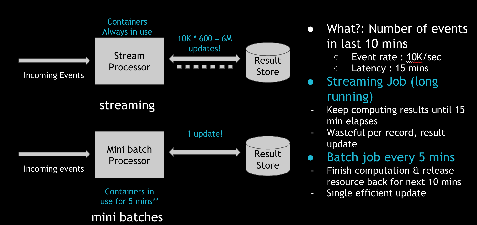
However, in the near-real-time context, these decisions may not be the best ones. To achieve the same effect, you can use short-lived containers and improve the overall resource utilization. In the figure above, the stream processor performs 6M updates over 15 minutes to the result store. But in the incremental processing model, we perform in-memory merge once and only one update to the result store, while using the containers for only five minutes. The incremental processing model is three times more CPU efficient, several magnitudes more efficient on updating of the result store. Basically, instead of waiting for work and eating up CPU and memory, the processing wakes up often enough to finish up pending work, grabbing resources on demand.
Built on top of existing SQL engines
Over time, a slew of SQL engines have evolved in the Hadoop/big data space (e.g., Hive, Presto, SparkSQL) that provide better expressibility for complex questions against large volumes of data. These systems have been deployed at massive scale and hardened over time in terms of query planning, execution, and so forth. On the other hand, SQL on stream processing is still in early stages. By performing incremental processing using existing, much more mature SQL engines in the Hadoop ecosystem, we can leverage the solid foundations that have gone into building them.
For example, joins are very tricky in stream processing, in terms of aligning the streams across windows. In the incremental processing model, the problem naturally becomes simpler due to relatively longer windows, allowing more room for the streams to align across a processing window. On the other hand, if correctness is more important, SQL provides an easier way to expand the join window selectively and reprocess.
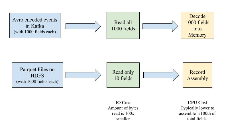
Another important advancement in such SQL engines is the support for columnar file formats like ORC/Parquet, which have significant advantages for analytical workloads. For example, joining two Kafka topics with Avro records would be much more expensive than joining two Hive/Spark tables backed by ORC/Parquet file formats. This is because with Avro records, you would end up de-serializing the entire record, whereas columnar file formats only read the columns in the record that are needed by the query. For example, if we are simply projecting out 10 fields out of a total 1,000 in a Kafka Avro encoded event, we still end up paying the CPU and IO cost for all fields. Columnar file formats can typically be smart about pushing the projection down to the storage layer.
Fewer moving parts
The famed Lambda architecture that is broadly implemented today has two components: speed and batch layers, usually managed by two separate implementations (from code to infrastructure). For example, Storm is a popular choice for the speed layer, and MapReduce could serve as the batch layer. In practice, people often rely on the speed layer to provide fresher (and potentially inaccurate) results, whereas the batch layer corrects the results of the speed layer at a later time, once the data is deemed complete. With incremental processing, we have an opportunity to implement the Lambda architecture in a unified way at the code level as well as the infrastructure level.
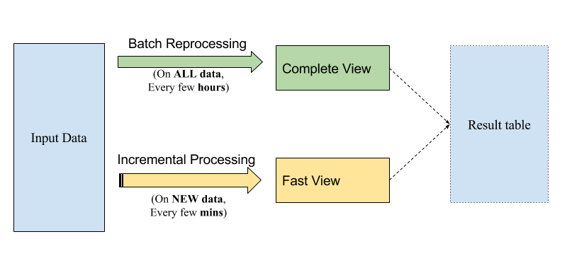
The idea illustrated in the figure above is fairly simple. You can use SQL, as discussed, or the same batch processing framework as Spark to implement your processing logic uniformly. The resulting table gets incrementally built by way of executing the SQL on the “new data” just like stream processing, to produce a “fast” view of the results. The same SQL can be run periodically on all of the data to correct any inaccuracies (remember, joins are tricky!), to produce a more “complete” view of the results. In both cases, we will be using the same Hadoop infrastructure for executing computations, which can bring down overall operational cost and complexity.
Challenges of incremental processing
Having laid out the advantages of an architecture for incremental processing, let’s explore the challenges we face today in implementing this in the Hadoop ecosystem.
Trade-off: Completeness vs. latency
In computing, as we traverse the line between stream processing, incremental processing, and batch processing, we are faced with the same fundamental trade-off. Some applications need all the data and produce more complete/accurate results, whereas some just need data at lower latency to produce acceptable results. Let’s look at a few examples.
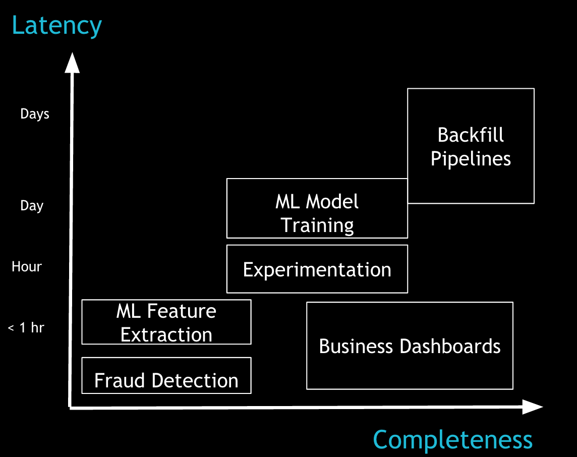
Figure 5 depicts a few sample applications, placing them according to their tolerance for latency and (in)completeness. Business dashboards can display metrics at different granularities because they often have the flexibility to show more incomplete data at lower latencies for recent times while over time getting complete (which also made them the marquee use-case for Lambda architecture). For data science/machine learning use cases, the process of extracting the features from the incoming data typically happens at lower latencies, and the model training itself happens at a higher latency with more complete data. Detecting fraud, on one hand, requires low-latency processing on the data available thus far. An experimentation platform, on the other hand, needs a fair amount of data, at relatively lower latencies, to keep results of experiments up to date.
The most common cause for lack of completeness is late-arriving data (as explained in detail in this Google Cloud Dataflow deck). In the wild, late data can manifest in infrastructure-level issues, such as data center connectivity flaking out for 15 minutes, or user-level issues, such as a mobile app sending late events due to spotty connectivity during a flight. At Uber, we face very similar challenges, as we presented at Strata + Hadoop World earlier this year.
To effectively support such a diverse set of applications, the programming model needs to treat late-arrival data as a first-class citizen. However, Hadoop processing has typically been batch-oriented on “complete” data (e.g., partitions in Hive), with the responsibility of ensuring completeness also resting solely with the data producer. This is simply too much responsibility for individual producers to take on in today’s complex data ecosystems. Most producers end up using stream processing on a storage system like Kafka to achieve lower latencies, while relying on Hadoop storage for more “complete” (re)processing. We will expand on this in the next section.
Lack of primitives for incremental processing
As detailed in this article on stream processing, the notions of event time versus arrival time and handling of late data are important aspects of computing with lower latencies. Late data forces recomputation of the time windows (typically, Hive partitions in Hadoop), over which results might have been computed already and even communicated to the end user. Typically, such recomputations in the stream processing world happen incrementally at the record/event level by use of scalable key-value stores, which are optimized for point lookups and updates. However, in Hadoop, recomputing typically just means rewriting the entire (immutable) Hive partition (or a folder inside HDFS for simplicity) and recomputing all jobs that consumed that Hive partition.
Both of these operations are expensive in terms of latency as well as resource utilization. This cost typically cascades across the entire data flow inside Hadoop, ultimately adding hours of latency at the end. Thus, incremental processing needs to make these two operations much faster so that we can efficiently incorporate changes into existing Hive partitions as well as provide a way for the downstream consumer of the table to obtain only the new changes.
Effectively supporting incremental processing boils down to the following primitives:
Upserts: Conceptually, rewriting the entire partition can be viewed as a highly inefficient upsert operation, which ends up writing way more than the amount of incoming changes. Thus, first-class support for (batch) upserts becomes an important tool to possess. In fact, recent trends like Kudu and Hive Transactions do point in this direction. The Google Mesa paper also talks about several techniques that can be applied in the context of ingesting quickly.
Incremental consumption: Although upserts can solve the problem of publishing new data to a partition quickly, downstream consumers do not know what data has changed since a point in the past. Typically, consumers learn this by scanning the entire partition/table and recomputing everything, which can take a lot of time and resources. Thus, we also need a mechanism to more efficiently obtain the records that have changed since the last time the partition was consumed.
With the two primitives above, you can support a lot of common-use cases by upserting one data set and then incrementally consuming from it to build another data set incrementally. Projections are the most simple to understand, as depicted in Figure 6.
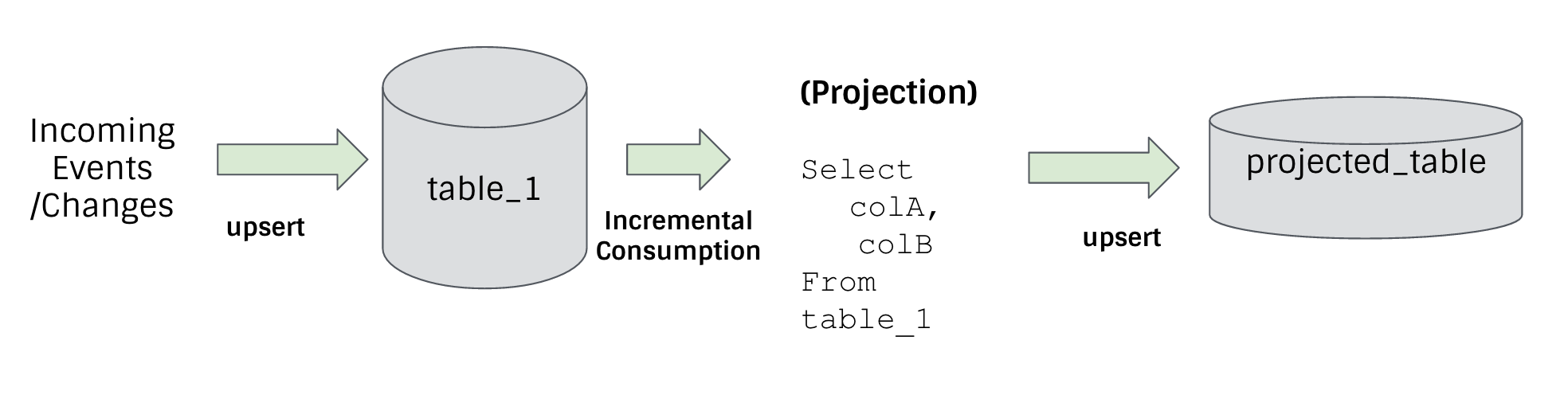
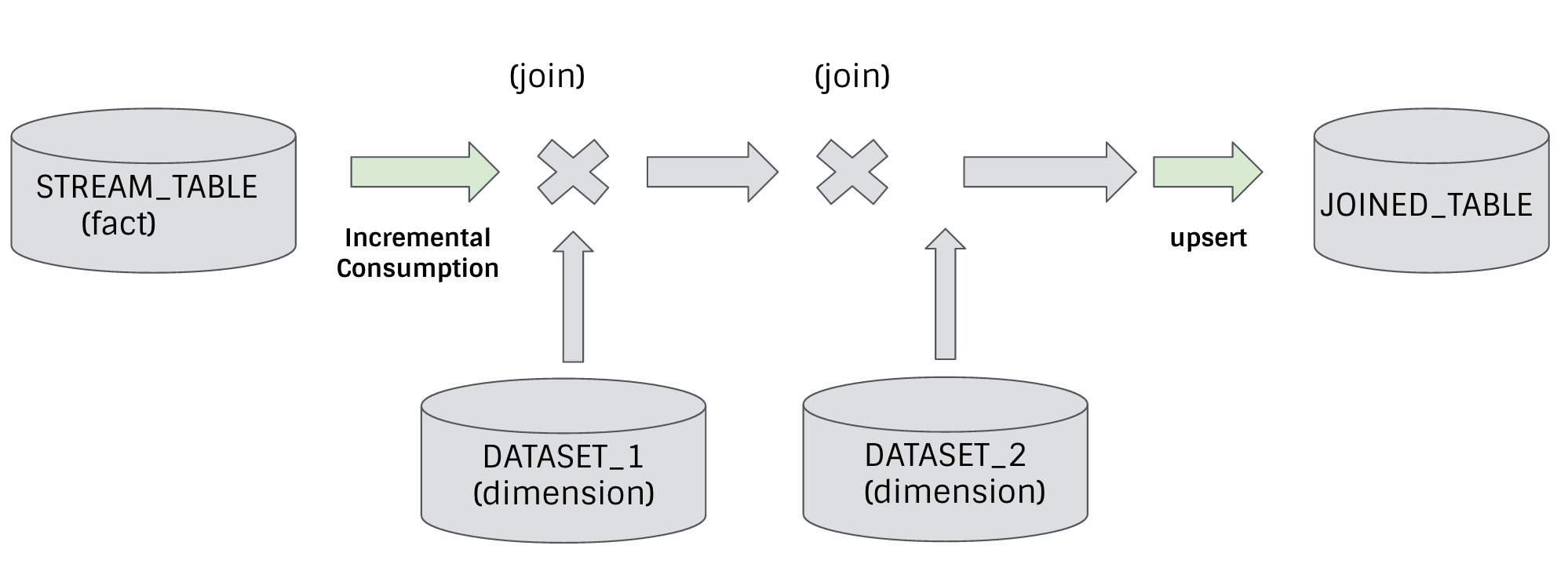
Borrowing terminology from Spark Streaming, we can perform simple projections and stream-data set joins much more efficiently at lower latency. Even stream-stream joins can be computed incrementally, with some extra logic to align windows.
This is actually one of the rare scenarios where we could save money with hardware while also cutting down the latencies dramatically.
Shift in mindset
The final challenge is not strictly technical. Organizational dynamics play a central role in which technologies are chosen for different use cases. In many organizations, teams pick templated solutions that are prevalent in the industry, and teams get used to operating these systems in a certain way. For example, typical warehousing latency needs are on the order of hours. Thus, even though the underlying technology could solve a good chunk of use cases at lower latencies, a lot of effort needs to be put into minimizing downtimes or avoiding service disruptions during maintenance. If you are building toward lower latency SLAs, these operational characteristics are essential. On the one hand, teams that solve low-latency problems are extremely good at operating those systems with strict SLAs, and invariably the organization ends up creating silos for batch and stream processing, which impedes realization of the aforementioned benefits to incremental processing on a system like Hadoop.
This is in no way an attempt to generalize the challenges of organizational dynamics, but is merely my own observation as someone who has spanned the online services powering LinkedIn as well as the data ecosystem powering Uber.
Takeaways
I would like to leave you with the following takeaways:
- Getting really specific about your actual latency needs can save you tons of money.
- Hadoop can solve a lot more problems by employing primitives to support incremental processing.
- Unified architectures (code + infrastructure) are the way of the future.
At Uber, we have very direct and measurable business goals/incentives in solving these problems, and we are working on a system that addresses these requirements. Please feel free to reach out if you are interested in collaborating on the project.