10 Elasticsearch metrics to watch
Track key metrics to keep Elasticsearch running smoothly.
Track key metrics to keep Elasticsearch running smoothly.
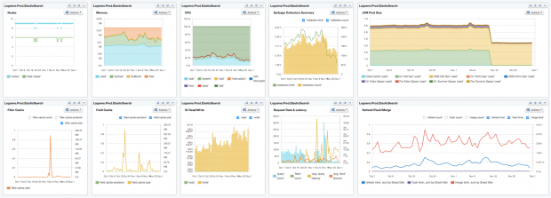
 SPM Dashboard (source: From Sematext’s SPM Performance Monitoring tool.)
Elasticsearch is booming. Together with Logstash, a tool for collecting and processing logs, and Kibana, a tool for searching and visualizing data in Elasticsearch (aka, the “ELK” stack), adoption of Elasticsearch continues to grow by leaps and bounds. When it comes to actually using Elasticsearch, there are tons of metrics generated. Instead of taking on the formidable task of tackling all-things-metrics in one blog post, I’ll take a look at 10 Elasticsearch metrics to watch. This should be helpful to anyone new to Elasticsearch, and also to experienced users who want a quick start into performance monitoring of Elasticsearch.
Most of the charts in this piece group metrics either by displaying multiple metrics in one chart, or by organizing them into dashboards. This is done to provide context for each of the metrics we’re exploring.

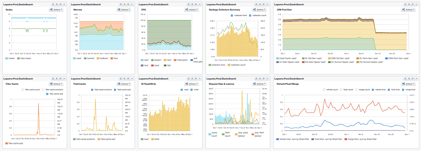
To start, here’s a dashboard view of the 10 Elasticsearch metrics we’re going to discuss:
Now, let’s dig into each of the 10 metrics one by one and see how to interpret them.
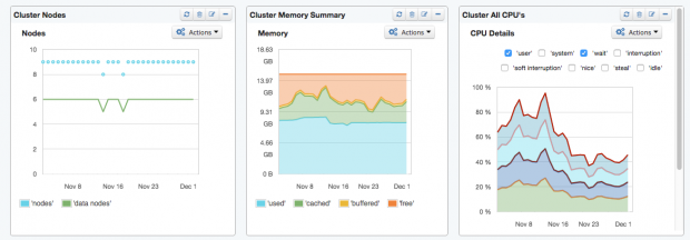
Like OS metrics for a server, the cluster health status is a basic metric for Elasticsearch. It provides an overview of running nodes and the status of shards distributed to the nodes.
Putting the counters for the shard allocation status together in one graph visualizes how the cluster recovers over time. Especially in the case of upgrade procedures with round-robin restarts, it’s important to know the time your cluster needs to allocate the shards.

The process of allocating shards after restarts can take a long time, depending on the specific settings of the cluster. Taking some control of shard allocation is given by the Cluster API.
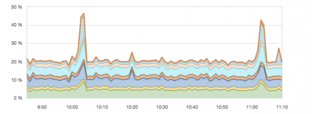
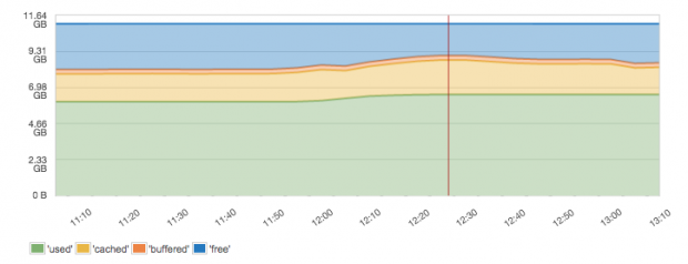
As with any other server, Elasticsearch performance depends strongly on the machine it is installed on. CPU, Memory Usage, and Disk I/O are basic operating system metrics for each Elasticsearch node.
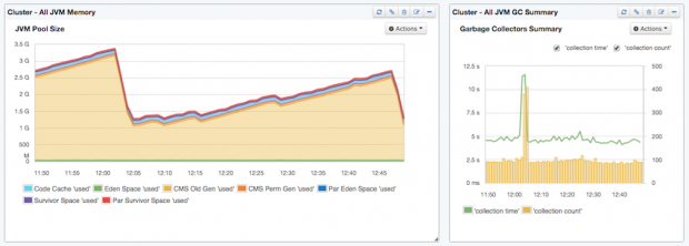
In the context of Elasticsearch (or any other Java application), it is recommended that you look into Java Virtual Machine (JVM) metrics when CPU usage spikes. In the following example, the reason for the spike was higher garbage collection activity. It can be recognized by the “collection count” because the time and and count increased.
The following graph shows a good balance. There is some spare memory and nearly 60% of memory is used, which leaves enough space for cached memory (e.g. file system cache). What you’d see more typically is actually a chart that shows no free memory. People new to looking at memory metrics often panic, thinking that having no free memory means the server doesn’t have enough RAM. That is actually not so. It is good not to have free memory. It is good if the server is making use of all the memory. The question is just whether there is any buffered and cached memory (this is a good thing) or if it’s all used. If it’s all used and there is very little or no buffered and cached memory, then indeed the server is low on RAM. Because Elasticsearch runs inside the Java Virtual Machine, JVM memory and garbage collection are the areas to look at for Elasticsearch-specific memory utilization.
Summary dashboard
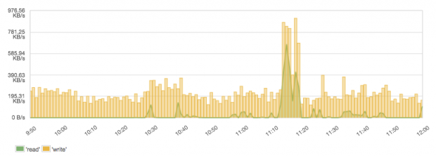
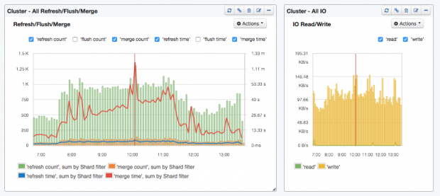
A search engine makes heavy use of storage devices, and watching the disk I/O ensures that this basic need gets fulfilled. As there are so many reasons for reduced disk I/O, it’s considered a key metric and a good indicator for many kinds of problems. It is a good metric to check the effectiveness of indexing and query performance. Distinguishing between read and write operations directly indicates what the system needs most in the specific use case. Typically, there are many more reads from queries than writes, although a popular use case for Elasticsearch is log management, which typically has high writes and low reads. When writes are higher than reads, optimizations for indexing are more important than query optimizations. This example shows a logging system with more writes than reads:
The operating system settings for disk I/O are a base for all other optimizations — tuning disk I/O can avoid potential problems. If the disk I/O is still not sufficient, countermeasures such as optimizing the number of shards and their size, throttling merges, replacing slow disks, moving to SSDs, or adding more nodes should be evaluated according to the circumstances causing the I/O bottlenecks. For example, while searching, disks get trashed if the indices don’t fit in the OS cache. This can be solved a number of different ways: by adding more RAM or data nodes, or by reducing the index size (e.g. using time-based indices and aliases), or by being smarter about limiting searches to only specific shards or indices instead of searching all of them, or by caching, etc.
Elasticsearch runs in a JVM, so the optimal settings for the JVM and monitoring of the garbage collector and memory usage are critical. There are several things to consider with regard to JVM and operating system memory settings:
bootstrap.mlockall=true in the Elasticsearch configuration file and the environment variable MAX_LOCKED_MEMORY=unlimited (e.g. in /etc/default/elasticsearch). To set swappiness globally in Linux, set vm.swappiness=1 in /etc/sysctl.conf. On Windows one can simply disable virtual memory.ES_HEAP_SIZE environment variable (-Xmx java option) and following these rules:
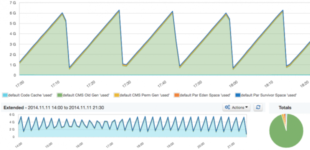
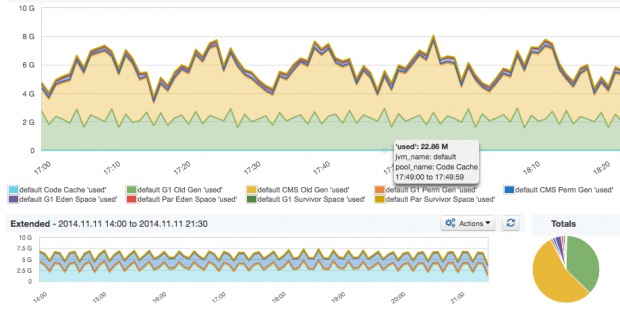
-Xms) equal to the maximum heap size (-Xmx), so there is no need to allocate additional memory during runtime. Example: ./bin/elasticsearch -Xmx16g -Xms16g-Xmx32g or higher results in the JVM using larger, 64-bit pointers that need more memory. If you don’t go over -Xmx31g, the JVM will use smaller, 32-bit pointers by using compressed Ordinary Object Pointers (OOPs).The report below should be obvious to all Java developers who know how JVM manages memory. Here, we see relative sizes of all memory spaces and their total size. If you are troubleshooting performance of the JVM (which one does with pretty much every Java application), this is one of the key places to check first, in addition to looking at the garbage collection and memory pool utilization reports (see graph “JVM pool utilization”). In the graph below, we see a healthy sawtooth pattern clearly showing when major garbage collection kicked in.
When we watch the summary of multiple Elasticsearch nodes, the sawtooth pattern is not as sharp as usual because garbage collection happens at different times on different machines. Nevertheless, the pattern can still be recognized, probably because all nodes in this cluster were started at the same time and are following similar garbage collection cycles.
The memory pool utilization graph shows what percentage of each pool is being used over time. When some of these memory pools, especially Old Gen or Perm Gen, approach 100% utilization and stay there, it’s time to worry. Actually, it’s already too late by then. You have alerts set on these metrics, right? When that happens you might also find increased garbage collection times and higher CPU usage, as the JVM keeps trying to free up some space in any pools that are (nearly) full. If there’s too much garbage collection activity, it could be due to one of the following causes:
ES_HEAP_SIZE). Lowering the utilized heap in Elasticsearch could theoretically be done by reducing the field and filter cache. In practice, it would have a negative impact to query performance by doing so. A much better way to reduce memory requirements for “not_analyzed” fields is to use the “doc_values” format in the index mapping/type definitions — it reduces the memory footprint at query time.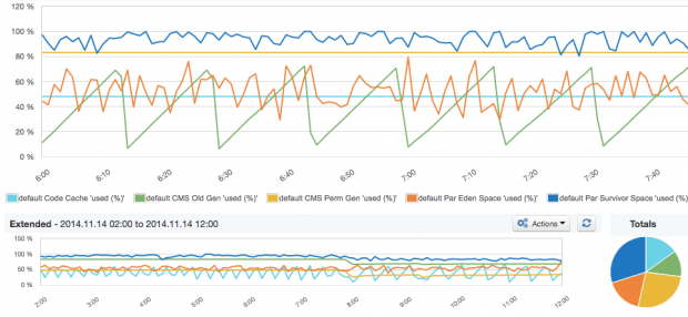
A drastic change in memory usage or long garbage collection runs may indicate a critical situation. For example, in a summarized view of JVM Memory over all nodes, a drop of several GB in memory might indicate that nodes left the cluster, restarted or got reconfigured for lower heap usage.
Summary dashboard
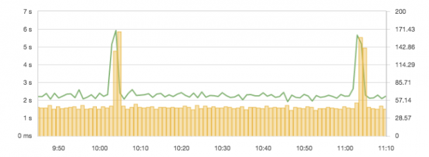
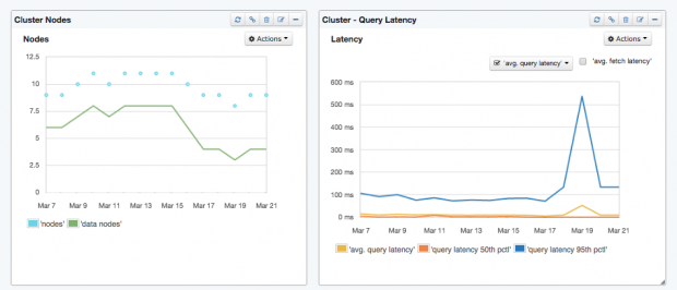
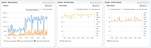
When it comes to search applications, the user experience is typically highly correlated to the latency of search requests. For example, the request latency for simple queries is typically below 100. We say “typically” because Elasticsearch is often used for analytical queries, too, and humans seem to still tolerate slower queries in scenarios. There are numerous things that can affect your queries’ performance — poorly constructed queries, improperly configured Elasticsearch cluster, JVM memory and garbage collection issues, disk IO, and so on. Needless to say, query latency is the metric that directly impacts users, so make sure you put some alerts on it. Alerts based on query latency anomaly detection will be helpful here. The following charts illustrate just such a case. A spike like the blue 95th percentile query latency spike will trip any anomaly detection-based alerting system worth its salt. A word of caution: query latencies that Elasticsearch exposes are actually per-shard query latency metrics. They are not latency values for the overall query.
Putting the request latency together with the request rate into a graph immediately provides an overview of how much the system is used and how it responds to it.
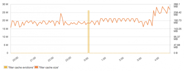
Most of the filters in Elasticsearch are cached by default. That means that during the first execution of a query with a filter, Elasticsearch will find documents matching the filter and build a structure called “bitset” using that information. Data stored in the bitset is really simple; it contains a document identifier and whether a given document matches the filter. Subsequent executions of queries having the same filter will reuse the information stored in the bitset, thus making query execution faster by saving I/O operations and CPU cycles. Even though filters are relatively small, they can take up large portions of the JVM heap if you have a lot of data and numerous different filters. Because of that, it is wise to set the “indices.cache.filter.size” property to limit the amount of heap to be used for the filter cache. To find out the best setting for this property, keep an eye on filter cache size and filter cache eviction metrics shown in the chart below.
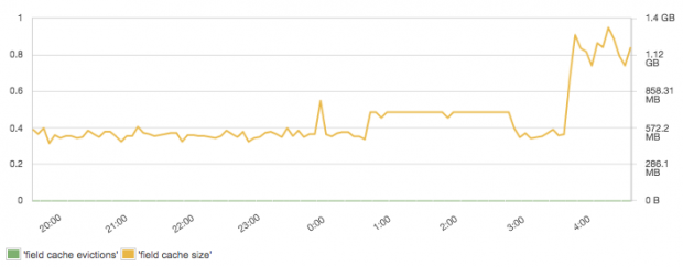
Field data cache size and evictions are typically important for search performance if aggregation queries are used. Field data is expensive to build — it requires pulling of data from disk into memory. Field data is also also used for sorting and for scripted fields. Remember that, by default (because of how costly it is to build it), field data cache is unbounded. This, of course, could make your JVM heap explode. To avoid nasty surprises, consider limiting the size of the field data cache accordingly by setting the “indices.fielddata.cache.size” property and keeping an eye on it to understand the actual size of the cache.
Summary dashboard
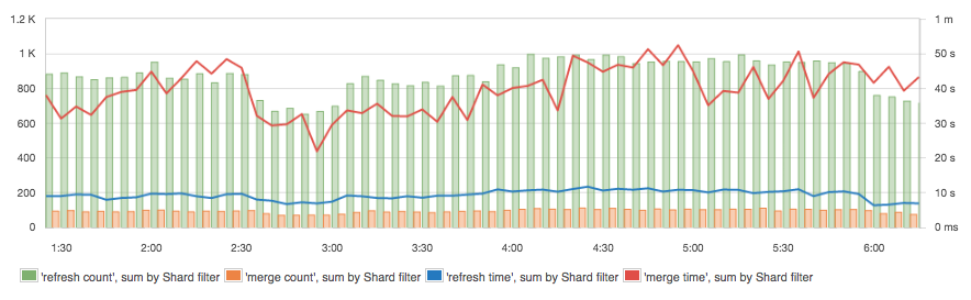
Several different things take place in Elasticsearch during indexing, and there are many metrics to monitor its performance. When running indexing benchmarks, a fixed number of records is typically used to calculate the indexing rate. In production, though, you’ll typically want to keep an eye on the real indexing rate. Elasticsearch itself doesn’t expose the rate itself, but it does expose the number of documents, from which one can compute the rate, as shown here:
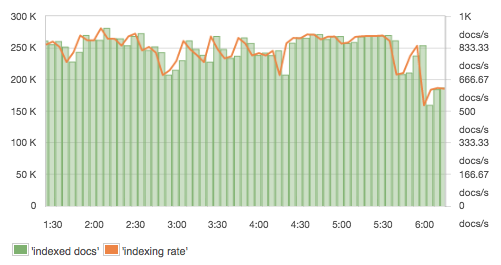
This is another metric worth considering for alerts and/or anomaly detection. Sudden spikes and dips in indexing rate could indicate issues with data sources. Refresh time and merge time are closely related to indexing performance, plus they affect overall cluster performance. Refresh time increases with the number of file operations for the Lucene index (shard). Reduced refresh times can be achieved by setting the refresh interval to higher values (e.g. from 1 second to 30 seconds). When Elasticsearch (really, Apache Lucene, which is the indexing/searching library that lives at the core of Elasticsearch) merges many segments, or simply a very large index segment, the merge time increases. This is a good indicator of having the right merge policy, shard, and segment settings in place. In addition, Disk I/O indicates intensive use of write operations while CPU usage spikes as well. Thus, merges should be as quick as possible. Alternatively, if merges are affecting the cluster too much, one can limit the merge throughput and increase “indices.memory.index_buffer_size” (to more than 10% on nodes with a small heap) to reduce disk I/O and let concurrently executing queries have more CPU cycles.
Segments merging is a very important process for the index performance, but it is not without side effects. Higher indexing performance usually means allowing more segments to be present and thus making the queries slightly slower.
Summary dashboard
So there you have it, the top Elasticsearch metrics to watch for those of you who find yourselves knee deep — or even deeper! — in charts, graphs, dashboards, etc. Elasticsearch is a high-powered platform that can serve your organization’s search needs extremely well, but, like a blazing fast sports car, you’ve got to know what dials to watch and how to shift gears on the fly to keep things running smoothly. Staying focused on these 10 metrics and corresponding analysis will keep you on the road to a successful Elasticsearch experience.
This post is part of a collaboration between O’Reilly and Sematext. See our statement of editorial independence.