 Grandstand (source: Pixabay)
 In recent years, the term “anomaly detection” (also referred to as “outlier detection”) has started popping up more and more on the internet and in conference presentations. This is not a new topic by any means, though. Niche fields have been using it for a long time. Nowadays, though, due to advances in banking, auditing, the Internet of Things (IoT), etc., anomaly detection has become a fairly common task in a broad spectrum of domains. As with other tasks that have widespread applications, anomaly detection can be tackled using multiple techniques and tools. This, of course, can cause a lot of confusion concerning what it’s for and how it works.
This article takes a look at how different types of neural networks can be applied to detect anomalies in time series data using Apache MXNet, a fast and scalable training and inference framework with an easy-to-use, concise API for machine learning, in Python using Jupyter Notebooks. By the end of this tutorial, you should:
- Know what anomaly detection is and the common techniques for solving it
- Be able to set up your MXNet environment
- See the difference between different types of networks, along with their strengths and weaknesses
- Load and preprocess the data for such a task
- Build network architectures in MXNet
- Train models using MXNet and use them for predictions
All the code and the data used in this tutorial can be found on GitHub.
Anomaly detection
When talking about any machine learning task, I like to start by pointing out that, in many cases, the task is really all about finding patterns. This problem is no different. Anomaly detection is a process of training a model to find a pattern in our training data, which we subsequently can use to identify any observations that do not conform to that pattern. Such observations will be called anomalies or outliers. In other words, we will be looking for a deviation from the standard pattern, something rare and unexpected.
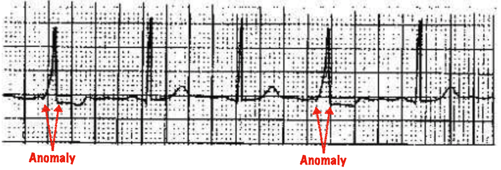
Figure 1 shows anomalies in a human heartbeat, indicating a medical syndrome.
An important distinction has to be made between anomaly detection and “novelty detection.” The latter turns up new, previously unobserved, events that still are acceptable and expected. For example, at some point in time, your credit card statements might start showing baby products, which you’ve never before purchased. Those are new observations not found in the training data, but given the normal changes in consumers’ lives, may be acceptable purchases that should not be marked as anomalies.
Anomalies can also be leveraged for multiple use cases:
- Predictive maintenance. In factories, or any kind of IoT environment, you can build a model using data gathered during normal execution modes and use it to predict imminent failure. This means no unplanned halts in production.
- Fraud detection. Financial institutions often use this technique to catch unexpected expenses: for example, if your credit card got stolen.
- Health care. Used for diagnostics, for instance.
- Cybersecurity. Ever wanted to catch all those intruders trying to hack into your system? Anomaly detection can help you.
Similarly, as mentioned before, a wide range of methods can be used to solve this problem. A few of the most popular include:
- Kalman filters, which use simple statistics
- K-nearest neighbors
- K-means clustering
- Deep learning-based autoencoders
Several problems arise when you try to use most of these algorithms. For instance, they tend to make specific assumptions about the data, and some do not work with multivariate data sets.
This is why today we will look into the last method—autoencoders—using two types of neural networks: multilayer perceptron and long-short-term-memory (LSTM) networks. For simplicity, this tutorial uses only a single feature, for which other methods might turn out just as good, but the great thing about neural nets is how good they are at modeling multivariate problems, which is what you’d probably want to do in production (especially when working with IoT time-series data, as in this example).
Autoencoders
The kind of networks we will discuss here go by many names: autoencoder; autoassociator; or, my personal favorite, Diabolo. The technique is a type of artificial neural network used for unsupervised learning of efficient codings. In plain English, this means it is used to find a different way of representing (encoding) our input data. Autoencoders are sometimes also used to reduce the dimensions of the data.
An autoencoder finds an approximation of the identity function (Id : X → X) through two steps:
- The encoder step, where the input data is transformed into an intermediate state
- The decoder step, which transforms it to match the number of input features

For the math buffs this can be described as two transitions:
\(\phi : X \rightarrow F\)
\(\psi : F \rightarrow X\)
Usually, autoencoders are trained by optimizing the mean square error between the output and input layers, where X is the input vector, Y is the output vector, and n is the number of elements:
\(Y = (\psi\circ\phi)X\)
\(MSE = \frac{1}{n}\sum^{n}_{i=1}(Y-X)^{2}\)
After we are done training our autoencoder, we need to set a threshold, which will decide whether we have predicted an anomaly or not. Depending on your exact use case and data, there are different ways to set this threshold—for example, based on a receiver operating characteristics (ROC) curve or F1 score. The higher the threshold you set, the longer it will take the system to detect an anomaly (and fewer will be detected, in some circumstances). In this tutorial, we will run predictions on our training data set after we are done training our model, calculate the error for each prediction, and find the mean and standard deviation for those errors. Everything higher than the third standard deviation will be marked as an anomaly.
System setup
We will need to first install a few tools before we can jump into data analysis and modeling. I highly recommend using some sort of a Python environment management system such as Anaconda or Virtualenv. This tutorial will use the latter.
-
Install Virtualenv. On most systems it should be as easy as calling
pip install virtualenv. - Create a new virtualenv environment by calling
virtualenv oreilly-anomaly. This will create a new folder called oreilly-anomaly in your current directory. - Activate the environment by calling
. oreilly-anomaly/bin/activate - Install Numpy, Pandas, Jupyter Notebook, and Matplotlib by running
pip install numpy pandas ipython jupyter ipykernel matplotlib - Install MXNet.
- Add the virtual env as a Jupyter kernel:
python -m ipykernel install --user --name=oreilly-anomaly - Run the notebook
jupyter notebook . - In Jupyter, choose oreilly as the kernel: Menu → Kernel → Change kernel → oreilly-anomaly
Data set
As mentioned in the introduction, anomaly detection can be used on data with labels or without labels from different industries. Today, we will use IoT-based data, which can be used for predictive maintenance. Predictive maintenance lets you, using machine data, predict ahead of time when an issue may occur. This has a number of advantages over scheduled maintenance. In traditional systems, you would have to either know your machines really well to know how often they need maintenance, or do frequent checks. Otherwise, there would be a chance of a failure.
The data was gathered using hardware sensors made by a Tokyo based startup, LP research. The sensors used this time can read up to 21 different values, including linear acceleration (rate of change in velocity without changing direction) in the X, Y, and Z dimensions. Today, for the sake of simplicity (and visualization), we will use only one feature: linear acceleration in X. In real life, you probably would want to use more, especially when using neural networks, as they are great at figuring out all the features by themselves.
Figure 3 shows sample data gathered about this feature.
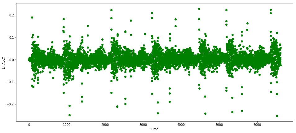
As you can see, the data is quite cyclical and already nicely scaled—this is not always the case. One thing to notice are the occasional spikes, which must be recognized as normal and not anomalous. We will need to make sure our model is smart enough to handle them.
Feed-forward networks
When working on a machine learning problem, starting with a simple solution and working your way up iteratively is always a good idea. Otherwise, you can get lost in the complexity from the start.
For that reason, we first will implement our autoencoder using one of the simplest possible types of neural networks, a multilayer perceptron (MLP). An MLP is a type of a feedforward neural network, meaning a network with no cycles—all the connections go forward (contrary to recurrent neural networks, which we will use in the next section). An MLP is a simple network with at least three layers: input, output, and at least one hidden layer between them. A feedforward autoencoder is a special type of MLP, where the number of neurons in the input layer is the same as the number of neurons in the output layer. A simple example appears in Figure 4.
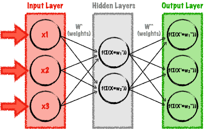
The main advantage of MLPs is that they are quite easy to model and fast to train. Also, a lot of research has been done using them, so they are fairly well understood.
When modeling an MLP, there are a few things you, as the creator, need to figure out, including:
- the number of hidden layers and number of neurons at each layer
- the type of activation function used in each neuron
- the optimizer used for training
All these choices will affect the results of your model. If you choose the wrong parameters, your network might not converge at all, take a long time to converge (for example, if you choose a bad optimizer or bad learning rate), overfit the real-life data, or underfit the real-life data.
Let’s go through the most important parts of the code.
Data preparation
We first read the data from our CSV files using the Pandas framework. This will return a Pandas Dataframe:
train_data_raw=pd.read_csv('resources/normal.csv')validate_data_raw=pd.read_csv('resources/verify.csv')
Now we want to extract the columns, which we will actually use for training and predictions:
feature_list=[" LinAccX (g)"]features=len(feature_list)train_data_selected=train_data_raw[feature_list].as_matrix()validate_data_selected=validate_data_raw[feature_list].as_matrix()
Before we start modeling our network, we need to do some more preprocessing. The major drawback of MLP networks is their lack of “memory.” Each record is treated as a separate entity during training and predictions. When dealing with time series, though, the dependency between observations is very important. A single spike in our data does not necessarily mean an anomaly: that depends on its surroundings.
To tackle this, we will create windowed records using a simple method, which will go record by record and append window - 1 records to the back of it (in our case, window will be set to 25, but this value should be based on your use case, frequency with which you are getting readings, and how fast you want your model to predict anomalies, potentially sacrificing accuracy). This new type of record will have window * features size and will mimic temporal dependency between between timesteps. If we wish to utilize the first window - 1 readings, though, we need to pad them to the appropriate length because MLP networks require a constant number of inputs. In this example, we will pad them with zeroes:
defprepare_dataset(dataset,window):windowed_data=[]foriinrange(len(dataset)):start=i+1-windowifi+1-window>=0else0observation=dataset[start:i+1,]to_pad=(window-i-1ifi+1-window<0else0)*featuresobservation=observation.flatten()observation=np.lib.pad(observation,(to_pad,0),'constant',constant_values=(0,0))windowed_data.append(observation)returnnp.array(windowed_data)
When building machine learning models, you don’t want to use all the data for training—this might leave you with a highly overfitted model. For this reason, it is normal to split the data into train and validation sets, and use both for evaluation during training. Normally, splitting the data is easy, but with time-series data, it gets a bit more complicated. This is because of the temporal dependency between records: the context in which each datapoint appears is very important. This is why in this tutorial, instead of randomly sampling the data, we will simply find a split point and use it to split the data into two subsets (80% of the data for training and 20% for testing):
rows=len(data_train)split_factor=0.8train=data_train[0:int(rows*split_factor)]test=data_train[int(rows*split_factor):]
Now we need to prepare a DataLoader object, which will feed the data in a batched manner to MXNet:
batch_size=256train_data=mx.gluon.data.DataLoader(train,batch_size,shuffle=False)test_data=mx.gluon.data.DataLoader(test,batch_size,shuffle=False)
This iterator will pass the training data in batches of 256 records. This is especially important if you’re running on the GPU—batches that are too big can quickly result in out-of-memory errors. On the other hand, batches that are too small will lengthen training time.
Modeling
The code for modeling is very brief thanks to the use of Apache Gluon, a high-level interface to MXNet.
Our model will be a sequence of blocks representing hidden layers. To make modeling easy, we will use the gluon.nn.Sequential for that:
model=gluon.nn.Sequential()withmodel.name_scope():
Adding hidden layers, activation functions, and a dropout layer now is a matter of simple MXNet method calls:
model.add(gluon.nn.Dense(16,activation='tanh'))# Adds a fully connected layer with 16 neurons and a tanh activationmodel.add(gluon.nn.Dropout(0.25))# Adds a dropout layer
This will feed the input, which we will pass later on to our model object, to the first hidden layer containing 16 neurons, pass it through an activation layer—in this case “tanh,” which not only is computationally cheaper than many other activation functions, but has also been shown to converge quickly and achieve high accuracy for MLP networks—and drop out a portion of our data so we do not overfit. In our network, we will pass the output of Dropout layer to another hidden layer and repeat the cycle two more times (hidden layer with 8 and 16 neurons—hidden layers should have fewer layers than the input one to find structure). Our final layer will not have any activation or dropouts after it and will be treated as the output layer.
Before modeling, we need to assign initial values to the network parameters (in this case, we are using the so-called Xavier initialization) and prepare a trainer object (here we are using the Adam optimizer:
model.collect_params().initialize(mx.init.Xavier(),ctx=ctx)trainer=gluon.Trainer(model.collect_params(),'adam',{'learning_rate':0.001})
For this problem (we are interested in calculating our loss as a difference between the output and input layers), we can use the gluon.loss.L2Loss to calculate the mean squared error for this:
L=gluon.loss.L2Loss()
Finally, we prepare an evaluation method, which will check how well our model does after each epoch:
defevaluate_accuracy(data_iterator,model,L):loss_avg=0.fori,datainenumerate(data_iterator):data=data.as_in_context(ctx)# Pass data to the CPU or GPUlabel=dataoutput=model(data)# Run batch through our networkloss=L(output,label)# Calculate the lossloss_avg=loss_avg*i/(i+1)+nd.mean(loss).asscalar()/(i+1)returnloss_avg
And train in a loop for a number of epochs:
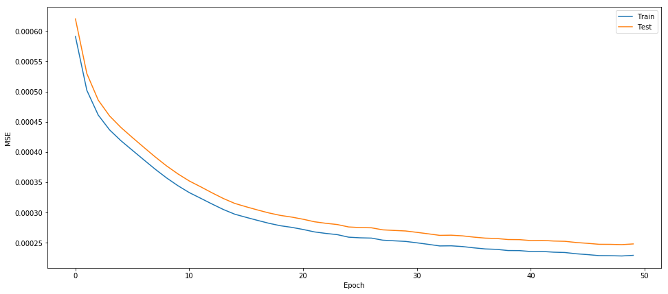
epochs=50all_train_mse=[]all_test_mse=[]# Gluon training loopforeinrange(epochs):fori,datainenumerate(train_data):data=data.as_in_context(ctx)label=datawithautograd.record():output=model(data)#Feed the data into our modelloss=L(output,label)#Compute the lossloss.backward()#Adjust parameterstrainer.step(batch_size)train_mse=evaluate_accuracy(train_data,model,L)test_mse=evaluate_accuracy(test_data,model,L)all_train_mse.append(train_mse)all_test_mse.append(test_mse)
Figure 5 shows how close the model works for our training data and validation data.
After fitting the model, we can feed new data to make predictions:
defpredict(to_predict,L):predictions=[]fori,datainenumerate(to_predict):input=data.as_in_context(ctx)out=model(input)prediction=L(out,input).asnumpy().flatten()predictions=np.append(predictions,prediction)returnpredictions
After calculating the MSE for all of our training data, we can set our threshold for anomalies:
threshold=np.mean(errors)+3*np.std(errors)
Finally, we can run predictions on a test data set, which was, in this case, prepared by programming the robot engine to simulate failure (another option would be to use statistics to generate erroneous data). Figure 6 shows the resulting anomalies in red.
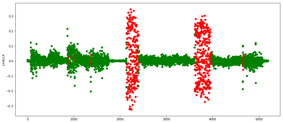
The robot was programmed so it would stutter around time 2,000 and just before 4,000, which the MLP diagnosed correctly.
As we can see, even though our training data set contained a lot of scattered points between 0.1 and 0.2, our network was smart enough to figure out that if there are multiple such readings together, there’s probably something wrong. We can also notice that it properly predicts that some readings with such values around time 1,000 are non-anomalous, but it also gets some of them wrong. We might need to tweak the parameters (dropout, regularization, or split type) a bit to get a better model.
The necessity of windowing our data set can be shown by running our script with window size 1 (see Figure 7):

We clearly see that the network does not respect any temporal structure and simply overfits to the majority of our training data set, which is approximately between [-1, 1]. All the scattered points outside that range are incorrectly marked as anomalies.
LSTM
Now that we have a working, basic, solution, let’s think about our problem a bit more. In the “data preparation” section of our MLP example, we mentioned that training record by record using MLP networks does not persist any previous information, and that this might be an issue in this case. This is because, in time-series analysis, the time dependency is often of great importance. Our windowing strategy was a poor man’s solution to this shortcoming in the MLP example.
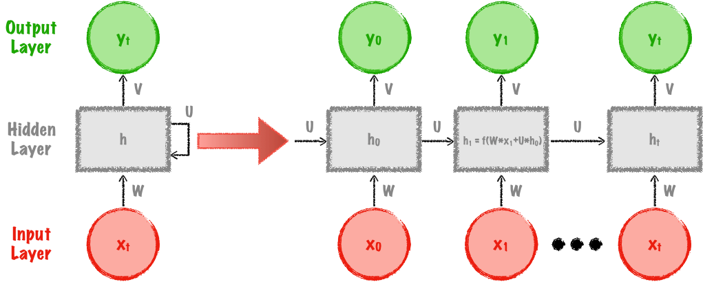
To overcome this shortcoming, we will look now into recurrent neural networks. As in FF nets, they will be built using neurons with activation functions, but the main difference is that they will also contain cycles. This will be achieved by feeding into our network not only the observation, but also some state from the previous run of the network. Figure 8 shows the architecture of an RNN.
The main issue with traditional RNNs is that, when using, for example, tanh or a similar activation layer in which output is always in the [-1,1] range, they encode a vast amount of information into a small output range. This makes learning long-term dependencies very challenging. For example, when building a model predicting the next word in a sentence, if the next word can be derived using only a few previous words, we will probably be fine. If, on the other hand, the context required is much broader (several sentences), we might not retain enough “long-term” information to be able to make a proper prediction.
For the math inclined, this is due to a phenomena called vanishing gradient and exploding gradient problems. In the latter case, the weights in our network can start growing exponentially, possibly becoming more important than they should. This problem could be solved by simple truncation or squashing of too high values. The former is a bigger problem, where some (or all) of our weights get smaller exponentially, sometimes becoming so small that the computation error on your machine might render them completely useless.
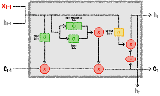
These problems led to the creation of so-called long short-term memory networks (LSTM). The basic idea behind LSTMs is that they, like traditional RNNs, have a chain-like structure and retain previous information, but at a more steady rate. Whereas vanilla RNNs have only one activation layer inside each cell, LSTMs use input (which decides what new information should be passed to the network), forget (which decides what information to forget and at what rate), and output gates to calculate the new state as shown in Figure 9.
By setting the number of outputs to the same value as the number of inputs, we can again obtain an autoencoder—this time one that remembers previous state on its own.
In contrast to our MLP example, we will not do any upfront data preprocessing. We will split the data into train and validation sets again, though. Gluon provides us with a bit different abstraction for data ingestion:
split_factor=0.8train=train_data_selected.astype(np.float32)[0:int(rows*split_factor)]validation=train_data_selected.astype(np.float32)[int(rows*split_factor):]train_data=mx.gluon.data.DataLoader(train,batch_size,shuffle=False)validation_data=mx.gluon.data.DataLoader(validation,batch_size,shuffle=False)
Wrapper classes make it easy to model even complex networks such as LSTM or, even better, sequences of LSTMs. The following code creates a sequence of stacked neural network blocks, initializes all the parameters using the Xavier initialization, generates an optimizer, and prepares a loss function:
model=mx.gluon.nn.Sequential()withmodel.name_scope():model.add(mx.gluon.rnn.LSTM(window,dropout=0.35))model.add(mx.gluon.rnn.LSTM(features))# Use the non default Xavier parameter initializermodel.collect_params().initialize(mx.init.Xavier(),ctx=ctx)# Use Adam optimizer for trainingtrainer=gluon.Trainer(model.collect_params(),'adam',{'learning_rate':0.01})# Similarly to previous example we will use L2 loss for evaluationL=gluon.loss.L2Loss()
Training in Gluon is performed in a simple for loop, looping the number of times specified by the variable epochs:
foreinrange(epochs):fori,datainenumerate(train_data):data=data.as_in_context(ctx).reshape((-1,features,1))label=datawithautograd.record():output=model(data)loss=L(output,label)loss.backward()trainer.step(batch_size)
This code will, for each epoch, use our training data batch by batch to calculate outputs using the model(data) call, then calculate the loss and update all the parameters using the trainer object. MSE results are shown in Figure 10.

In this case, both MSE values converge really fast to 0. This might mean we are overfitting our model and should probably tweak some parts of our network design.
Using the same technique as in our previous example, we can obtain a threshold value and run predictions on our test set, which produce the results shown in Figure 11.
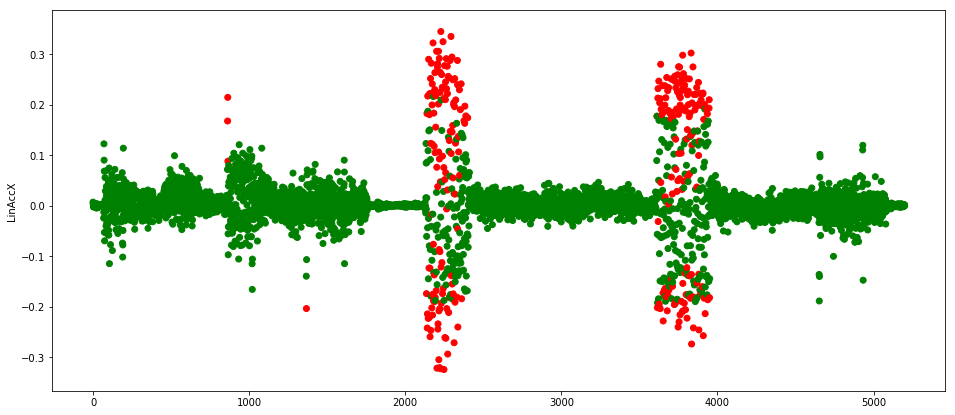
As we can see this time, the network is not predicting all of the readings of the erroneous cycles as anomalies, but it did get enough right for us to detect a problem with the machine.
Further improvements
Even though we were able to create seemingly useful models in this tutorial, there are still several important aspects we did not have time to cover:
- Data preparation. Depending on your data set, you might need to explore additional data preparation steps. For example, it is often a good idea to normalize your time-series data for neural networks. In other cases, you will need to encode your features—for example when you have categorical features.
- Network architecture optimization. Different use cases will require a different number of hidden layers, activation functions, regularizations, optimizers, dropout layers, etc.
- If you go through the LSTM Gluon doc and the LSTM diagram again, you will notice that each sample in an LSTM problem can be defined as a sequence of observations. Similarly, as in the MLP example, we could use our windowing method to make it so every observation contained several readings and insert that into our LSTM network. In this case, the network could potentially make more use of the temporal dependency between readings, while the input to the network would still be only of size features.
- Different train/validation split strategies and automated model evaluation. We evaluated our model only by plotting and checking a sample test set. In the real world, you will want to prepare labeled test data sets (for example, using statistics) and use some kind of metric, such as prediction and recall, to see in an automated fashion how well your model is performing.
Conclusions
In this tutorial, we tackled the problem of anomaly detection in time-series IoT data. As we now see, anomaly detection is a very broad problem, where different use cases require different techniques both for data preparation and modeling. We explored two robust approaches: feed-forward neural networks and long short-term memory networks, each having advantages and disadvantages. FFNs are faster (5.5 sec for 50 epochs vs 33 sec for 25 epochs on an NVidia 1080 GPU) but require a bit more planning and preparation upfront, whereas LSTMs are a bit slower but also smarter. Deep neural networks prove to be really good at finding structure and dependencies, but in return require at least basic knowledge of how to structure them. Finally, we see the importance of frameworks, such as Apache MXNet, to make this difficult task more approachable.