 Kaleidoscope (source: PublicDomainPictures.net)
 The Wolfram Language is a high-level, functional programming language. It’s the language behind Mathematica, but Wolfram Cloud and Wolfram Desktop are other products in which you can use it. The language itself includes a built-in neural net framework, which is currently implemented using MXNet as a back end.
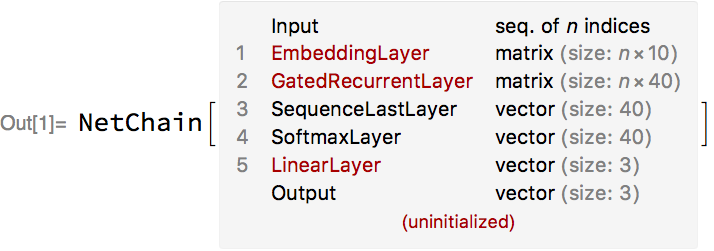
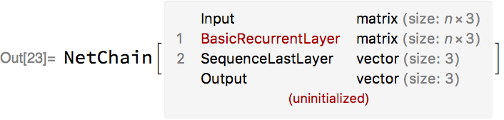
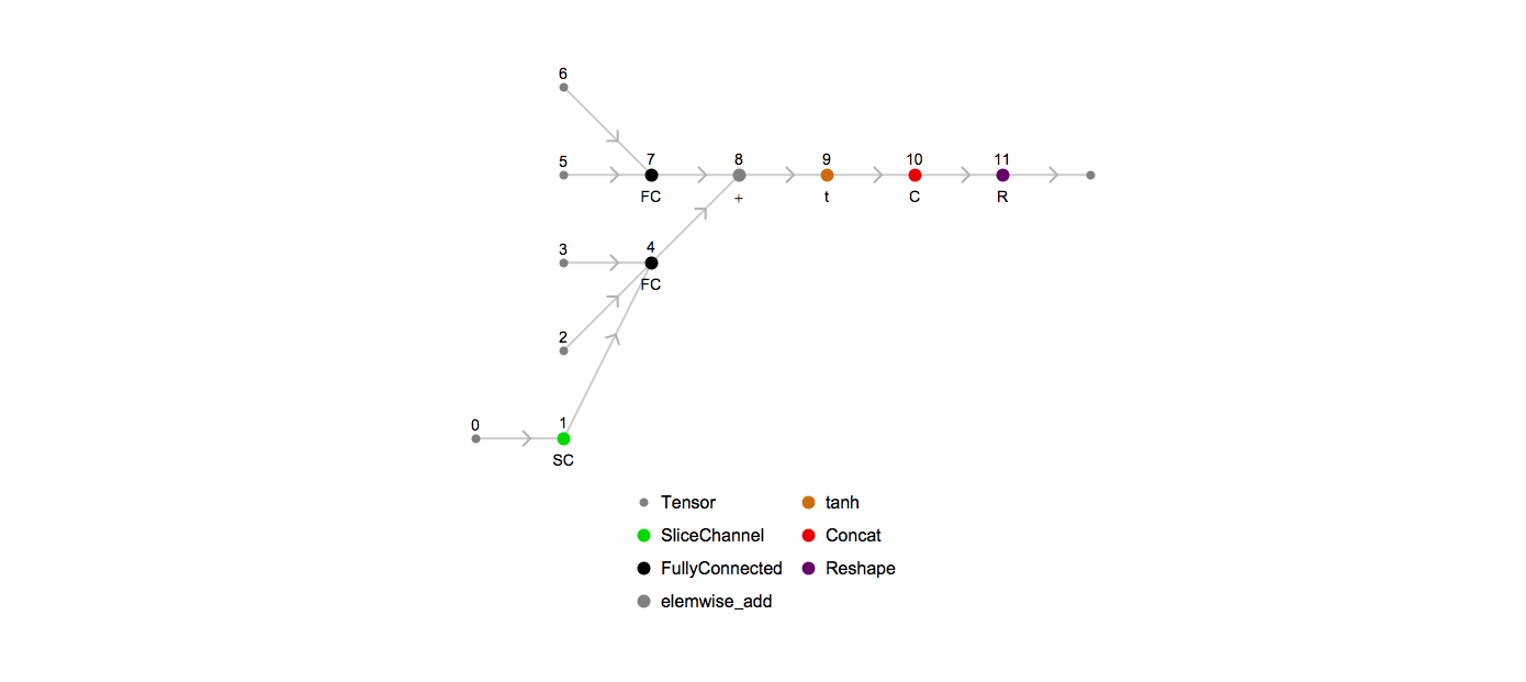
To give a sense of what a typical neural net looks like in the Wolfram Language, here is a recurrent net whose input is a sequence of integers and whose output is a vector of three numbers:

The aim of this post will be threefold: to explain why MXNet was chosen as a back end, to show how the Wolfram Language neural net framework and MXNet can interoperate, and finally to explain in some technical detail how Wolfram Language uses MXNet to train nets that take sequences of arbitrary length (like the example above).
Choosing MXNet
In 2015, we at Wolfram decided to integrate a neural net framework into the Wolfram Language. We wanted to target a level of abstraction closer to wrappers like Lasagne (released 2014) or Keras (released March 2015) than Theano (the underlying framework on which Lasagne and Keras were built). In addition, the idea of building on top of an existing framework was very appealing: we could focus most of our efforts on writing the best possible high-level framework, and share the work of improving the low-level back end with a much larger community.
The framework landscape was much simpler then, consisting of Torch, Theano, and Caffe, and a few less well-known frameworks such as MXNet’s progenitor CXXNet. However, a key design principle of the Wolfram Language is maximal platform independence: it should work on x86, iOS, and ARM (the Wolfram Language is shipped with the Raspberry Pi). However:
In addition, these frameworks were not designed to be easily wrapped by other languages. For example, much of Torch is written in Lua. Did we want to run Torch/Lua in a separate process, alongside the Wolfram Language kernel? (But then sharing large arrays between the two becomes hard to make efficient.) Or should we try to embed Lua directly in the Wolfram Kernel? (But then we would have to deal with memory issues and various other gotchas.)
The reason for this situation was perfectly understandable: these were frameworks of the researcher, by the researcher, for the researcher! And they were fantastic at what they did. MXNet was built with a different emphasis: immediate cross-platform support and the ability to be easily wrapped by other languages.

Furthermore, MXNet was architected with distributed training foremost amongst its concerns, appropriate for industrial-scale training. Finally, MXNet supported some visionary features: mixing symbolic and dynamic execution (finding its apotheosis in MXNet’s new Python interface, Gluon), and so-called “mirroring” feature that allows users to make flexible tradeoffs between computation time and memory usage.
For all of these reasons, we immediately switched our nascent efforts to MXNet when it was released in late 2015. Now, two years on, we have been very pleased with this decision. And after the demise of Theano, MXNet is now the only major framework that is developed by a diverse community and not limited to a single major corporation, but still supported by big players such as Amazon and Apple. This is a very healthy situation for a framework serving as common multi-organization infrastructure.
Interoperability
The Wolfram Language neural net framework is interoperable with MXNet, as it is easy to export and import nets to and from MXNet. To see a simple example, let’s define a net in the Wolfram Language:

Next, let’s export the net to the MXNet Symbol JSON file format. If the net has parameters, then these will also be exported as an MXNet parameter file:


Let’s look at the generated JSON:

{"nodes":[{"op":"null","name":"Input","attr":{},"inputs":[]},{"op":"sin","name":"1$0","attr":{},"inputs":[[0,0,0]]},{"op":"tanh","name":"2$0","attr":{},"inputs":[[1,0,0]]},{"op":"_Mul","name":"3$0","attr":{},"inputs":[[2,0,0],[1,0,0]]},{"op":"_Plus","name":"4$0","attr":{},"inputs":[[3,0,0],[2,0,0]]}],"arg_nodes":[0],"heads":[[4,0,0]],"attrs":{"mxnet_version":["int",905]}}
This can be imported into MXNet’s Python interface via:
importmxnetasmxsym=mx.symbol.load('example.json')
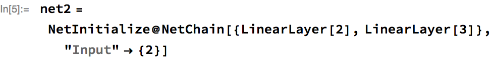
Next up, let’s look at a net containing initialized arrays. Let’s create a simple chain of two linear layers and initialize the weights and biases:
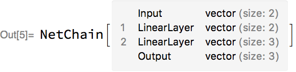
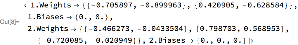
We can extract the weights of the first layer and display them as output:


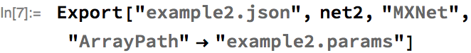
Both the parameters and the network structure can be exported to MXNet:

Import just the MXNet parameter file:

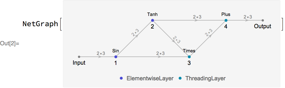
We also provide a number of utilities for working with MXNet Symbols. For example, you can visualize the directed acyclic graph, encoded in an MXNet Symbol file:

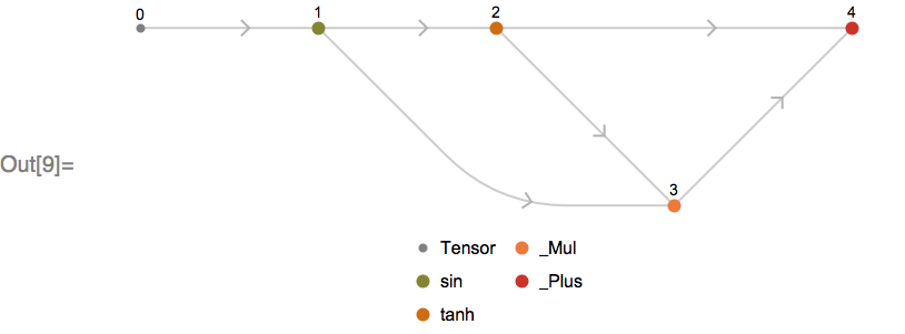
Or represent the symbol as a Graph object, suitable for computation in the Wolfram Language:

The Wolfram Language has a full suite of functionality for analyzing these graphs. For example, we can compute a measure of the “depth” of the network, being the longest path from the input to the output of the network:

This interoperability between the Wolfram Language and MXNet allows MXNet users to freely work in the Wolfram Language for a part of a project, and easily move back to MXNet for the other part. And there are a number of unique features of the Wolfram Language framework that might interest MXNet users. The particular feature we will look at next is our extensive support for nets that process variable-length sequences, or “dynamic dimensions” as these are sometimes called.
Variable-length sequences and MXNet
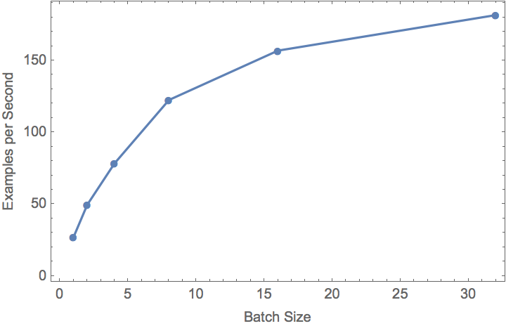
Many applications, such as language translation, speech recognition, and timeseries processing, involve inputs that do not have a fixed length. A common requirement in deep learning frameworks, including MXNet, is that all examples in a training batch be the same size (for the framework aficionado: two notable exceptions are DyNet and CNTK). In MXNet, most tensor operations are batched, by which we mean they operate on an input tensor consisting of the data for multiple examples and produce another tensor consisting of the outputs for those examples. Batched operations are used because they often produce order-of-magnitude training speedups over non-batched versions of the same operations on common hardware (such as GPUs):
The problem, therefore, is to group multiple sequences of varying lengths into a single tensor to allow the sequences to be processed together by batched operations. One simple solution to this problem is to “pad” the inputs to the length of the longest sequence. An example of padding a sequence of vectors is shown below (padding in red):
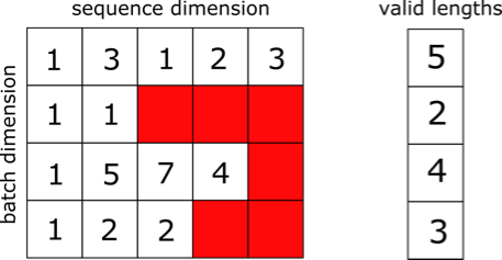
This has two drawbacks:
First: padding to the maximum length means that layers (such as recurrent layers) need to evaluate every example as though its length is the longest sequence length, resulting in potentially significant wasted computation. This is particularly serious for training on sequences of very different lengths.
Second: adding padding changes the learning problem, as the net now needs to learn how to ignore the padding. For problems such as language translation, a special padding token is often used, further changing the learning problem.
MXNet (and TensorFlow) partially deal with both problems via bucketing: they group examples of similar length together, before padding them. Then very little computation is wasted per batch. It also minimizes the amount of padding the net must learn to ignore, although the padding values are still treated as part of the learning problem. Note that this is done irrespective of whether so-called “static” or “dynamic” graphs are used.
There are other approaches that allow variable-length sequences to be processed in batches, such as by collapsing the sequence and batch dimensions entirely and “packing” the sequences one after another. But these have their own drawbacks.
In the Wolfram Language neural net framework, we completely automate the bucketing process (both for training and for evaluation on large sets of inputs). In addition, we completely remove any notion of padding from the learning problem. To illustrate this, we will first show an example of training a net on variable-length inputs in the Wolfram Language neural net framework, and then explain how this is implemented in terms of MXNet operations.
Variable-length sequences in the Wolfram Language
Let’s consider a simple example of training a net that operates on variable-length sequences. We will train a net to take a simple arithmetic sum, represented by a string (e.g., 43+3), and predict the output value (e.g., 46). First, we must generate some training data:
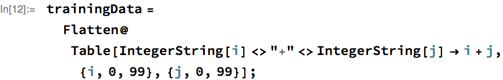
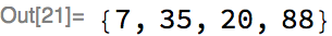
We generated 10,000 examples, but let’s look at four at random:


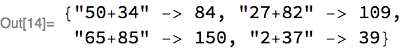
Notice that the inputs in these examples can be of different lengths, ranging from length 3 (e.g., “0+0”) to length 5 (“25+25”).
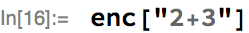
Next, we need to define an encoder that splits the string into characters, and encodes the characters into one-hot vectors that we can feed to the net:

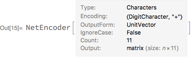
We’ve given a simple alphabet that we will use to translate each string into a vector of integers:

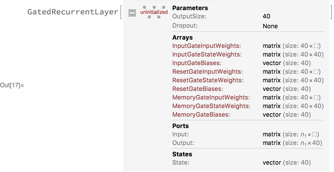
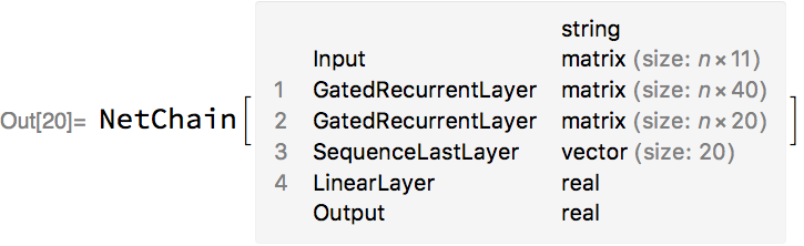
Now, we’ll define a net that takes a sequence of vectors and processes it with a stack of gated recurrent layers (GatedRecurrentLayer). Each recurrent layer takes as input a sequence of vectors and produces as output another sequence of vectors. Here’s one such layer:

After the recurrent layers, we use SequenceLastLayer (similar to SequenceLast in MXNet) to extract the last vector of the sequence, and use this as a feature representing the sequence. This is then fed into a LinearLayer (or FullyConnected in MXNet) to predict the numeric value of the sum:
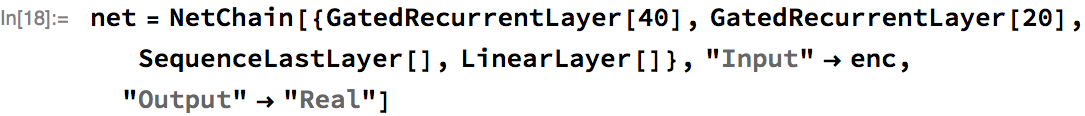
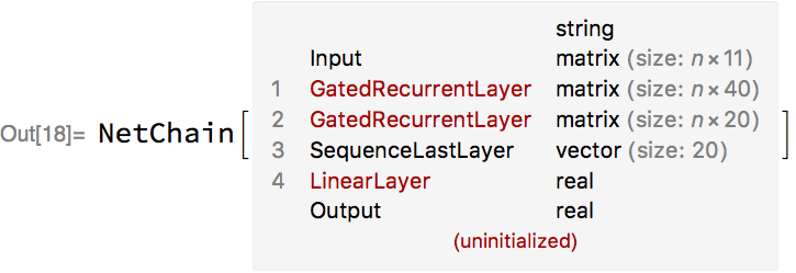
The net is formatted so that we can see each layer and the type of tensor that it produces. This makes it very easy to see at a glance how the input tensors are transformed to produce the output tensors.
Let’s evaluate the net on a random example using randomly initialized parameters:


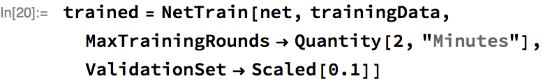
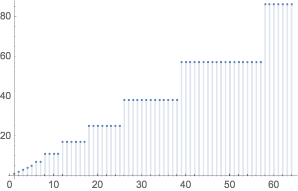
Obviously, it produces a random-looking output, but we haven’t trained it yet. So, let’s train for two minutes, and use 10% of the training set as a validation set:
Here’s the trained net evaluated on a set of inputs, where we’ve rounded the actual prediction to the nearest integer:

In this example, the user did not have to worry about doing any padding at all, even though the inputs were of different lengths. How is this magic achieved using MXNet operations? A rough summary of how it is done in the Wolfram Language:
- Standard bucketing: group training data into similar sequence-length groups, padding the data to have the same length in each bucket. Each of these buckets has its own MXNet Symbol and MXNet Executor, which share memory with all the others.
- Use arrays of integers to track the actual lengths of the variable length sequences as they flow through the net.
- Construct per-bucket MXNet Symbols , whose outputs have no dependence on padded values. This is done using a variety of tricks, including using MXNet operations that enable runtime variable-length sequence manipulation (such as SequenceLast, SequenceReverse and SequenceMask). These ops depend on the input sequence lengths tracked in Step 2.
Let us look more closely at how bucketing is done and how padding-invariant Symbols are constructed.
Bucketing
When it comes time to train or evaluate a net that operates on variable length inputs, Wolfram Language will create a permutation that partitions the inputs into buckets containing examples of similar length. It then creates MXNet Executors that are specialized for each of these lengths, transparently switching between them as needed to process each batch. Where possible, the compilation step between top-level framework and MXNet will be entirely bypassed, and existing executors will be reused through a process called “reshaping,” in which the input and output arrays are simply resized to be smaller or larger.
Each bucket corresponds to a family of similar sequence lengths, and each bucket is associated to a single MXNet Executor that shares all parameters with executors for other buckets, as well as sharing memory buffers used for temporary arrays, etc. We use logarithmic rounding of bucket sizes to ensure that the number of executors does not grow too quickly as longer and longer sequences are encountered. A given input sequence length will be rounded up to the next largest bucket size before the corresponding executor is retrieved or created:

Because each bucket still covers a range of sequence lengths, we must still pad the examples up to the bucket length. Most frameworks stop here, and rely on the network to learn how to deal with the padding. Next, we’ll explain how this dependence on padding is completely removed in the Wolfram Language neural net framework.
Important bucketing detail: Unrolling recurrent nets
For most layers, the underlying MXNet operation that can be used is the same for different sizes of input tensor. However, this is not always the case for recurrent layers. This section will look at how recurrent layers are handled for different sequence lengths.
Recurrent layers like long short-term memory (LSTM) and gated recurrent unit (GRU) process the input sequentially, maintaining an internal “state” as they go along (if you’re new to recurrent nets, a great visual introduction can be found here). The recurrence that gives recurrent neural networks (RNNs) their name has an important consequence: when producing a computational graph to implement an RNN, the number of nodes required will depend on the length of the input sequence:
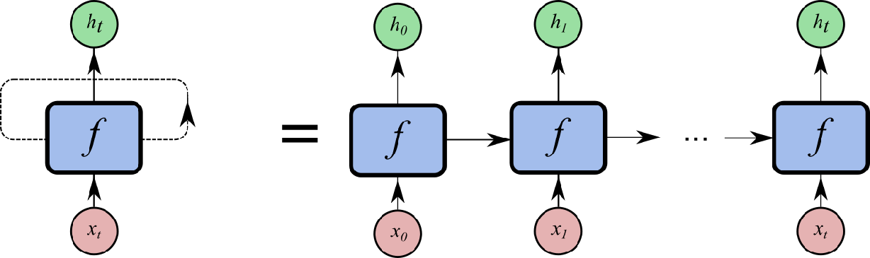
This means that if we implement an RNN naively out of simpler operations, we can’t use a single computational graph to evaluate an RNN on a short sequence, such as “2+2”, and a longer sequence, such as “55+55”. Each length requires its own graph. Producing these graphs by choosing a given length is known as “unrolling.”
MXNet does have an RNN op that implements many useful types of recurrent layer as a single operation that operates on a length of sequence, which would seem to avoid the need to do unrolling.
Unfortunately, the RNN op as it stands today has no CPU implementation, because it began life as a simple wrapper for the NVIDIA cuDNN RNN API. Additionally, there are variations of the common recurrent layers that employ other forms of regularization or different activation functions that are not currently supported by the cuDNN API. And perhaps most importantly, the Wolfram Language allows users to define their own recurrent layers by using “higher-order operators” like NetFoldOperator. These custom recurrent layers can’t, in general, be supported by a built-in MXNet operation.
So, in general, if we want a recurrent net to support multiple sequence lengths, the framework will need to automatically unroll the net into a graph that is specialized to operate on a given input length. To see this in a concrete example, consider a BasicRecurentLayer:

In the above example, the option "Input" -> {"Varying", 3} specifies that the first dimension of the input is varying, meaning it can be any size, and the second dimension is of size 3. Hence the input accepts any sequence of size-3 vectors, indicated in the display form as n x 3.
In fact, we can have multiple inputs with varying dimensions. Here is a more complex net that transforms two input sequences using recurrent layers, and then adds their final states:
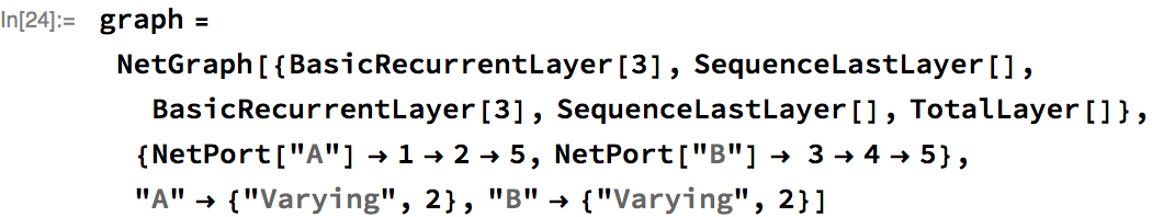
Let’s randomly initialize the weights of this network, and then apply it to input sequences of length 2 and 3 respectively:


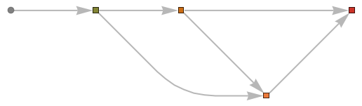
Returning to the topic of unrolling, we can examine what the underlying MXNet computation graph looks like for the above chain for a particular sequence length. To visualize the unrolled graph, we will use an internal utility, and choose the unrolled sequence length to be 3:

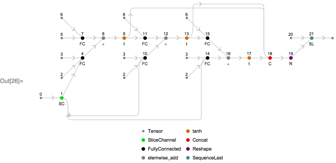
Looking at this graph, the input tensor (labeled as 0) is split via node 1 into three sub-tensors (one per element in the length-3 sequence), which are fed into three successive recurrent units that involve the same weight matrices (labeled as 2, 3 and 6). The final sequence is then formed by concatenating the output tensors together via node 18.
Node 21 is an MXNet SequenceLast op, which takes the last element of each sequence based on sequence lengths passed to it at runtime via node 20. This is one example of how sequence-length invariant symbols are constructed.
Here’s an animation of how the unrolled graph changes as the sequence length increases:

Achieving general padding invariance
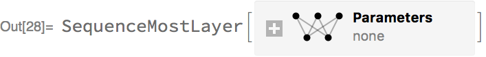
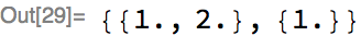
The first major principle for achieving padding invariance is to track sequence lengths inside the MXNet Symbol. If a net returns a sequence, then we can use these lengths to trim off any padding. Consider a layer that removes the last element of a sequence, SequenceMostLayer:

Applying this layer to a batch of two sequences of scalars:

The MXNet Symbol of this is:

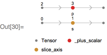
This Symbol takes a batch of sequence lengths (node 2) and adds -1 via _plus_scalar to obtain a new batch of sequence lengths (as the output sequence has one less element than the input sequence). This new sequence length is used to trim padding from the output as a post-processing step.
The second major principle is that we require layer-specific handling of variable sequences, and, in general, a high-level layer in the Wolfram Language must often go to special effort to avoid depending on padding. The three most common classes of layers are the following:
First: any Wolfram Language layers whose underlying MXNet operations have the property that the non-padded part of their output depends only on the non-padded portion of their input immediately support variable length sequences without any special effort. An example is the MXNet operation sin, or indeed any elementwise operation. In the Wolfram Language, this means that layers like ElementwiseLayer or ThreadingLayer, which are built out of primitives that have this property, immediately support variable length inputs.
Second: some MXNet operations explicitly take a vector of sequence lengths as one of their inputs. An example is SequenceReverse, which corresponds directly to the Wolfram Language layer SequenceReverseLayer. Other MXNet examples are CTCLoss, SequenceLast, and SequenceMask..
Third: are operations, such as summing the values in a sequence, that will depend, in general, on padding values. For many of these operations, SequenceMask can be used alongside the operation to make the operation compatible with variable-length sequences. As an example, consider the MXNet Softmax operation applied across a vector of fixed length, corresponding to SoftmaxLayer in Wolfram Language:

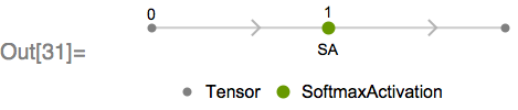
The graph consists of a single primitive MXNet operation, as we’d expect.
Now let’s look at a Softmax applied over a vector of varying length—note that this will evaluate only in the upcoming 11.3 version of the Wolfram Language:

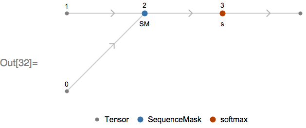
We can see the SequenceMask MXNet operation has been introduced. This operation, along with a second input containing the sequence lengths (node 1), has been used to replace the padded values of the input with the minimum 32-bit float value (approximately -1×1037). This replacement has the effect of preventing the padded portions of the input contributing to the computation of the softmax, as when exponentiated, these values underflow and do not contribute to the normalization factor of the softmax.
Similar tricks are being used to add variable-length sequence support to a growing list of layers including CrossEntropyLossLayer, SequenceAttentionLayer, AggregationLayer, and the up-coming CTCLossLayer.
Conclusion
We’ve looked at how we came to choose MXNet as the back end for the Wolfram Language neural net framework, how high-level nets compile down to MXNet graphs, and how unrolling and bucketing are used to implement RNNs that can efficiently operate on variable-length sequences. We’ve also looked at how existing MXNet layers can be adapted to work correctly on variable-length sequences using masking.
Hopefully this has made clear the value of a high-level framework like that provided by the Wolfram Language: users can focus on the meaning of their network, and simply by specifying a particular dimension as “Varying,” can have a network that processes inputs of any dynamic length, without requiring any other changes to their code. MXNet provides the basic set of building blocks that make it possible to efficiently provide this level of abstraction to our users.