Compressing and regularizing deep neural networks
Improving prediction accuracy using deep compression and DSD training.
 "Directed Differentiation of Multipotential Human Neural Progenitor Cells." (source: National Institutes of Health on Wikimedia Commons)
Deep neural networks have evolved to be the state-of-the-art technique for machine learning tasks ranging from computer vision and speech recognition to natural language processing. However, deep learning algorithms are both computationally intensive and memory intensive, making them difficult to deploy on embedded systems with limited hardware resources.
To address this limitation, deep compression significantly reduces the computation and storage required by neural networks. For example, for a convolutional neural network with fully connected layers, such as Alexnet and VGGnet, it can reduce the model size by 35x-49x. Even for fully convolutional neural networks such as GoogleNet and SqueezeNet, deep compression can still reduce the model size by 10x. Both scenarios results in no loss of prediction accuracy.

Learn faster. Dig deeper. See farther.
Current training methods are inadequate
Compression without losing accuracy means there’s significant redundancy in the trained model, which shows the inadequacy of current training methods. To address this, I’ve worked with Jeff Pool, of NVIDIA, and Sharan Narang, of Baidu, and Peter Vajda, of Facebook, to develop the Dense-Sparse-Dense (DSD) training, a novel training method that first regularizes the model through sparsity-constrained optimization, and improves the prediction accuracy by recovering and retraining on pruned weights. At test time, the final model produced by DSD training still has the same architecture and dimension as the original dense model, and DSD training doesn’t incur any inference overhead. We experimented with DSD training on mainstream CNN / RNN / LSTMs for image classification, image caption and speech recognition, and found substantial performance improvements.
In this article, we first introduce deep compression, and then introduce dense-sparse-dense training.
Deep compression
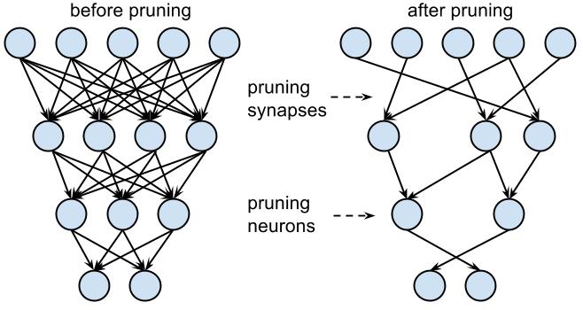
The first step of deep compression is Synaptic pruning. The human brain has the process of pruning inherently. 5x synapses are pruned away from infant age to adulthood.
Does a similar rule apply to artificial neural networks? The answer is yes. In early work, network pruning proved to be a valid way to reduce the network complexity and overfitting. This method works on modern neural networks as well. We start by learning the connectivity via normal network training. Next, we prune the small-weight connections: all connections with weights below a threshold are removed from the network. Finally, we retrain the network to learn the final weights for the remaining sparse connections. Pruning reduced the number of parameters by 9x and 13x for AlexNet and the VGG-16 model.
The next step of deep compression is weight sharing. We found neural networks have really high tolerance to low precision: aggressive approximation of the weight values does not hurt the prediction accuracy. As shown in Figure 2, the blue weights are originally 2.09, 2.12, 1.92 and 1.87; by letting four of them share the same value, which is 2.00, the accuracy of the network can still be recovered. Thus we can save very few weights, call it “codebook,” and let many other weights share the same weight, storing only the index to the codebook.
The index could be represented with very few bits; for example, in the below figure, there are four colors, thus only two bits are needed to represent a weight, as opposed to 32 bits originally. The codebook, on the other side, occupies negligible storage. Our experiments found this kind of weight-sharing technique is better than linear quantization, with respect to the compression ratio and accuracy trade-off.
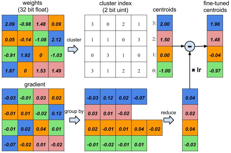
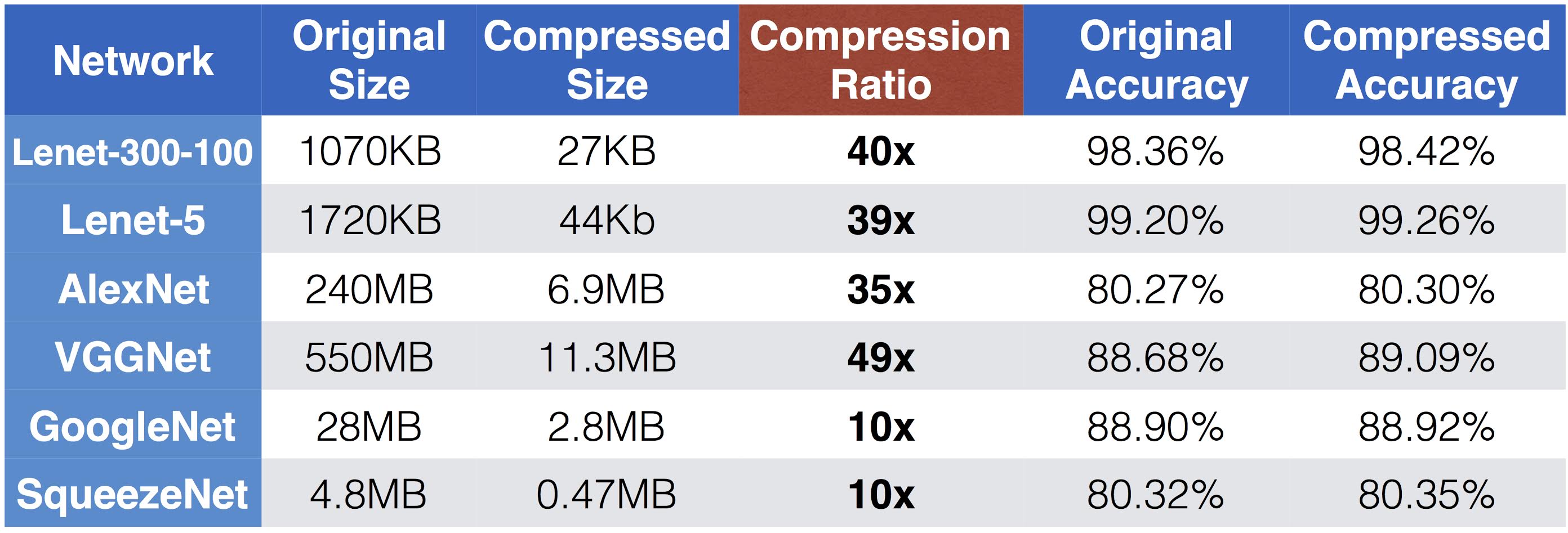
Figure 3 shows the overall result of deep compression. Lenet-300-100 and Lenet-5 are evaluated on MNIST data set, while AlexNet, VGGNet, GoogleNet, and SqueezeNet are evaluated on ImageNet data set. The compression ratio ranges from 10x to 49x—even for those fully convolutional neural networks like GoogleNet and SqueezeNet, deep compression can still compress it by an order of magnitude. We highlight SqueezeNet, which has 50x less parameters than AlexNet but has the same accuracy, and can still be compressed by 10x, making it only 470KB. This makes it easy to fit in on-chip SRAM, which is both faster and more energy efficient to access than DRAM.
We have tried other compression methods such as low-rank approximation based methods, but the compression ratio isn’t as high. A complete discussion can be found in the Deep Compression paper.
DSD training
The fact that deep neural networks can be aggressively pruned and compressed means that our current training method has some limitation: it can not fully exploit the full capacity of the dense model to find the best local minima, yet a pruned, sparse model that has much fewer synapses can achieve the same accuracy. This brings a question: can we achieve better accuracy by recovering those weights and learn them again?
Let’s make an analogy to training for track racing in the Olympics. The coach will first train a runner on high-altitude mountains, where there are a lot of constraints: low oxygen, cold weather, etc. The result is that when the runner returns to the plateau area again, his/her speed is increased. Similar for neural networks, given the heavily constrained sparse training, the network performs as well as the dense model; once you release the constraint, the model can work better.
Theoretically, the following factors contribute to the effectiveness of DSD training:
- Escape Saddle Point: One of the most profound difficulties of optimizing deep networks is the proliferation of saddle points. DSD training overcomes saddle points by a pruning and re-densing framework. Pruning the converged model perturbs the learning dynamics and allows the network to jump away from saddle points, which gives the network a chance to converge at a better local or global minimum. This idea is also similar to Simulated Annealing. While Simulated Annealing randomly jumps with decreasing probability on the search graph, DSD deterministically deviates from the converged solution achieved in the first dense training phase, by removing the small weights and enforcing a sparsity support.
- Regularized and Sparse Training: The sparsity regularization in the sparse training step moves the optimization to a lower-dimensional space where the loss surface is smoother and tends to be more robust to noise. More numerical experiments verified that both sparse training and the final DSD reduce the variance and lead to lower error.
- Robust re-initialization: Weight initialization plays a big role in deep learning. Conventional training has only one chance of initialization. DSD gives the optimization a second (or more) chance during the training process to re-initialize from more robust sparse training solutions. We re-dense the network from the sparse solution, which can be seen as a zero initialization for pruned weights. Other initialization methods are also worth trying.
- Break Symmetry: The permutation symmetry of the hidden units makes the weights symmetrical, thus prone to co-adaptation in training. In DSD, pruning the weights breaks the symmetry of the hidden units associated with the weights, and the weights are asymmetrical in the final dense phase.
We examined several mainstream CNN/RNN/LSTM architectures on image classification, image caption, and speech recognition data sets, and found that this dense-sparse-dense training flow gives significant accuracy improvement. Our DSD training employs a three-step process: dense, sparse, dense; each step is illustrated in Figure 4.
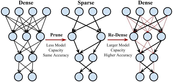
- Initial dense training: The first D-step learns the connectivity via normal network training on the dense network. Unlike conventional training, however, the goal of this D step is not to learn the final values of the weights; rather, we are learning which connections are important.
- Sparse training: The S-step prunes the low-weight connections and retrains the sparse network. We applied the same sparsity to all the layers in our experiments, thus there’s a single hyperparameter: the sparsity. For each layer we sort the parameters, the smallest N*sparsity parameters are removed from the network, converting a dense network into a sparse network. We found that a sparsity ratio of 50%-70% works very well. Then, we retrain the sparse network, which can fully recover the model accuracy under the sparsity constraint.
- Final Dense Training: The final D step recovers the pruned connections, making the network dense again. These previously pruned connections are initialized to zero and retrained. Restoring the pruned connections increases the dimensionality of the network, and more parameters make it easier for the network to slide down the saddle point to arrive at a better local minima.
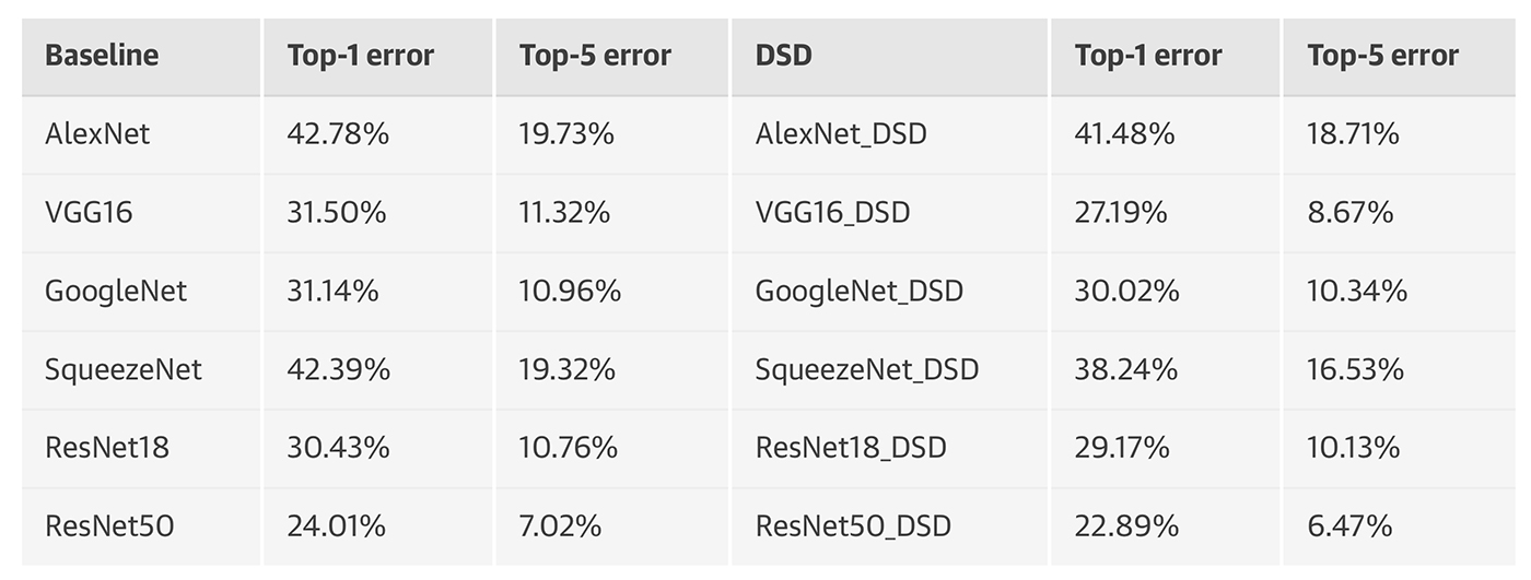
We applied DSD training to different kinds of neural networks on data sets from different domains. We found that DSD training improved the accuracy for all these networks compared to neural networks that were not trained with DSD. The neural networks are chosen from CNN, RNN, and LSTMs; the data sets are chosen from image classification, speech recognition, and caption generation. The results are shown in Figure 5. DSD models are available to download at DSD Model Zoo.
Generating image descriptions
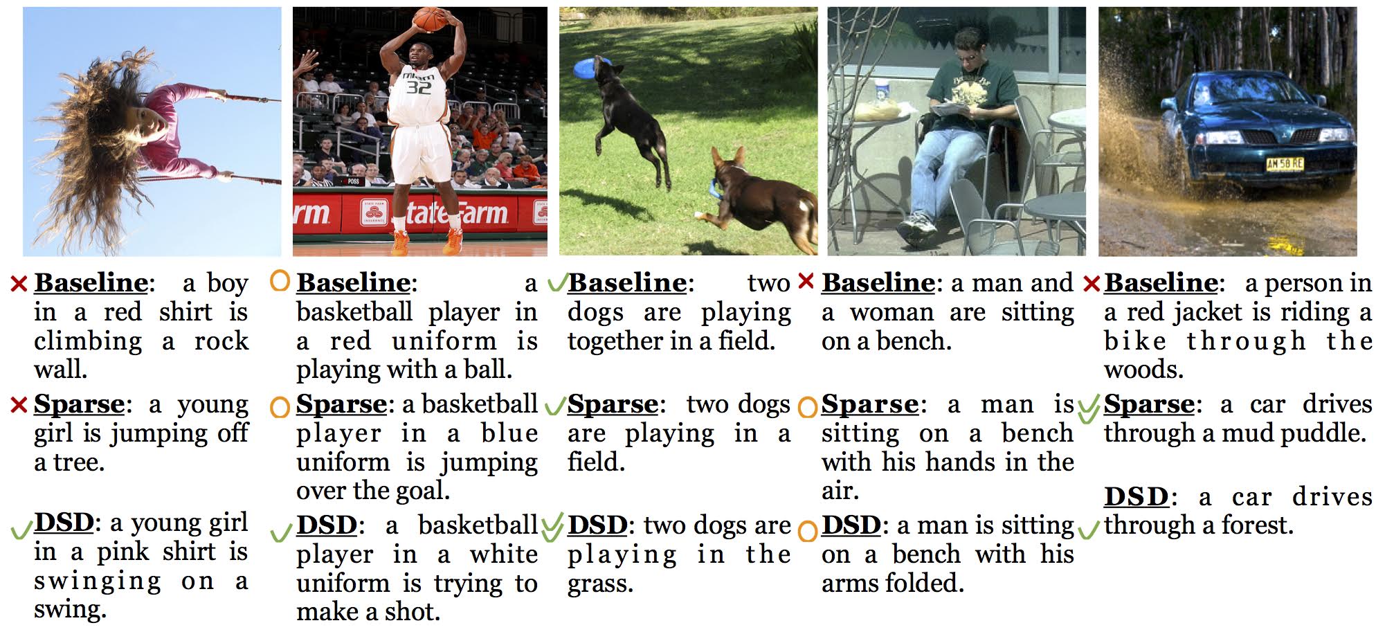
We visualized the effect of DSD training on an image caption task (see Figure 6). We applied DSD to NeuralTalk, an LSTM for generating image descriptions. The baseline model fails to describe images 1, 4, and 5. For example, in the first image, the baseline model mistakes the girl for a boy, and mistakes the girl’s hair for a rock wall; the sparse model can tell that it’s a girl in the image, and the DSD model can further identify the swing.
In the the second image, DSD training can tell the player is trying to make a shot, rather than the baseline, which just says he’s playing with a ball. It’s interesting to notice that the sparse model sometimes works better than the DSD model. In the last image, the sparse model correctly captured the mud puddle, while the DSD model only captured the forest from the background. The good performance of DSD training generalizes beyond these examples, and more image caption results generated by DSD training are provided in the appendix of this paper.
Advantages of sparsity
Deep compression, for compressing deep neural networks for smaller model size, and DSD training for regularizing neural networks, are both techniques that utilize sparsity and achieve a smaller size or higher prediction accuracy. Apart from model size and prediction accuracy, we looked at two other dimensions that take advantage of sparsity: speed and energy efficiency, which is beyond the scope of this article. Readers can refer to EIE for further references.