Fishing for graphs in a Hadoop data lake

Graphs in the sense of linked data with vertices and edges are everywhere these days: social networks, computer networks, and citations, to name but a few. And the data is generally big. Therefore, a lot of folks have huge amounts of data in graph format, typically sitting in some Hadoop file system as a table file for the vertices and a table file for the edges. At the same time, there are very good analytics tools available, such as Spark with GraphX and the more recent GraphFrames libraries. As a consequence, people are able to run large-scale graph analytics, and thus derive a lot of value out of the data they have.

Spark is generally very well suited for such tasks—it offers a great deal of parallelism and makes good use of distributed resources. Thus, it works great for workloads that essentially inspect the whole graph. But, there is even more information to be found in your graphs by inspecting many small regions of the graph, and I’ll present concrete examples in this article. For such smaller and rather ad-hoc workloads, it is not really worthwhile to launch a big job in Spark, even if you have to run many of them. Therefore, we will explore another possibility, which is to extract your graph data—or at least a part of it—and store it in a specialized graph database, which is then able to run many relatively small ad-hoc queries with very low latency. This makes it possible to use the results in interactive programs or graphical user interfaces.

In this article, I’ll explain this approach of exploring small regions of a graph using specialized graph databases in detail by discussing graph queries and capabilities of graph databases, while presenting concrete use cases in real-world applications. As an aside, we’ll take a little detour to discuss multi-model databases, which further enhances the possibilities of the presented approach.

This article targets data scientists, people doing data analytics, and indeed anybody who has access to large amounts of graph data and would like to get more insight out of it. We in the community believe that exploring these graphs very quickly, using many local queries with graph or multi-model databases, is eminently feasible and greatly enhances our toolboxes to gain insight into our data.

Graph data and “graphy” queries

Our tour through graph data land begins with a few examples of graphs in real-world data science.

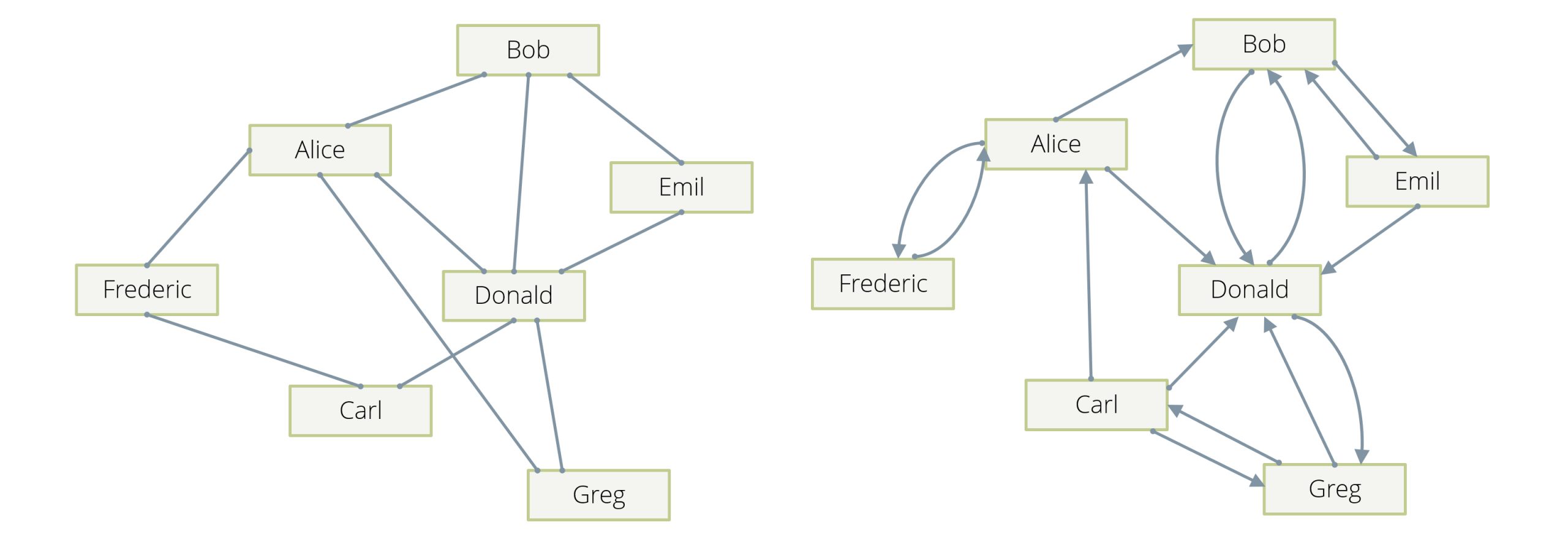
The prototypical example is a social network, in which the people in the network are the vertices of our graph, and their “friendship” relation is described by the edges: whenever person A is a friend of a person B, there is an edge in the graph between A and B, so edges are “undirected” (see Example 1 in Figure 1). Note that in another incarnation of this example, edges can be “directed” (see Example 2 in Figure 1)—an edge from A to B can, for example, mean that A “follows” B, and this can happen without B following A. Usually in these examples, there will be one (or at most two in the follower case) edge(s) between any two given vertices.

Another example is computer networks, in which the individual machines and routers are the vertices and the edges describe direct connectivity between vertices. A variation of this is that the edges are actually happening in network connections, which will usually carry a timestamp. In this latter case, there can be many different edges between two given machines over time.

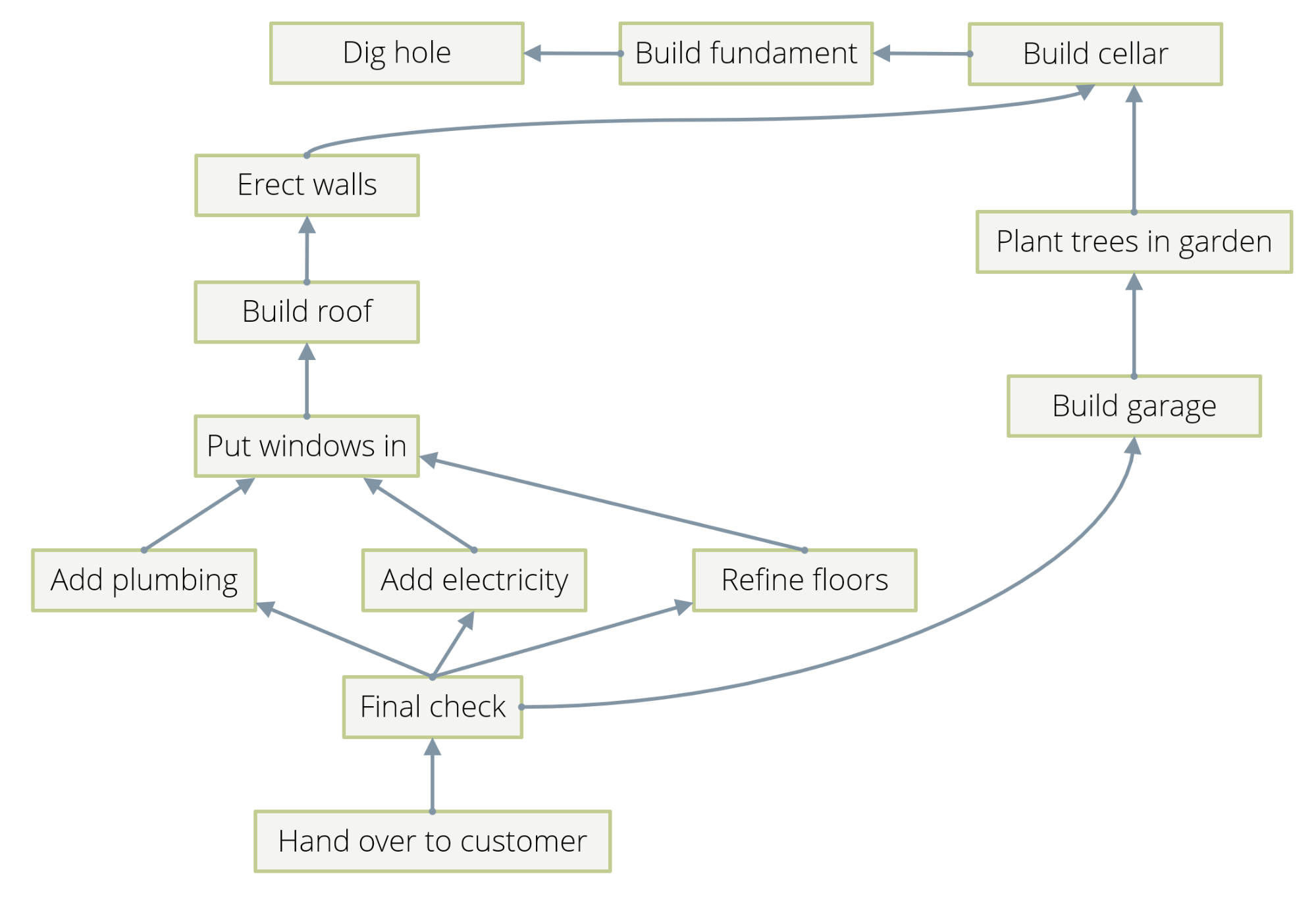
Examples are actually so abundant that there is a danger to bore you by presenting too many in too great a detail. So, I’ll just mention in passing that dependency chains between events can be described by directed edges between them. See Example 3 in Figure 2 for an illustration. Hierarchies can be described by directed edges, which describe the ancestor/descendant relation. Citations between publications are naturally the edges of a graph.

One distinguishes “directed” and “undirected” graphs. In the former, each edge has a direction; it goes from one vertex A to another one B, and not the other way around. Dependency chains, hierarchies, and citations are examples of directed graphs. In an undirected graph, an edge does not have a direction and simply links two vertices in a symmetric fashion. The friendship relation between two people is usually symmetrical and can therefore be modeled by an undirected graph.

Mathematically, every relation between two sets—X and Y—is a directed graph, in which the elements of the union of the two sets are the vertices, and two elements have one edge between them if and only if they are in relation. However, as can already be seen in some of the above examples, directed graphs are an even more general concept because there can be multiple different edges between two given vertices, and because the edges can carry additional data like timestamps. This is why there are so many real-world examples of graphs.

Graphy queries

For data scientists, the immediate challenge is: “In what ways can graph data be analyzed, such that we get answers to interesting questions?” And on a more technical level: “How can we actually perform these analyses efficiently?”

We have seen that every relation is a graph, so every “relational” question is a graph question, too. But these are not the most “graphy” questions. Let’s look deeper into a few of the above examples.

In a social graph, typical questions are (apart from the basic question of who is friends with whom):

• Find somebody in the “friendship vicinity.” That is, given a person P, explore the friends, the friends of these friends, and so on to find another person with a certain property.
• Find all people reachable with at most k friendship steps.
• Find a shortest chain of friendship steps from person P to person Q.

In a hierarchy, one might ask:

• What are all the recursive descendants?
• What is the closest ancestor?
• What is the closest common ancestor of two nodes?

For a graph of network connections between hosts, sensible problems are:

• Find a certain pattern of connectivity to detect intrusions.
• Find other machines (potentially with multiple hops) to which some machine connected that has visited this given site.

In a graph of websites and links between them one might:

• Rank web pages by “importance,” assuming that important sites have more links pointing to them (Google’s PageRank).
• Find connected components.
• Compute connectivity measures.
• Find distances from one site to all others.

Note that the questions in the last example are fundamentally different from the others. The problems described there all consider the whole graph and essentially ask for a result for each vertex. Let’s call these “global” problems. All other problems essentially started in some place in the graph (“given a person,” “… of a node,” etc.) and explored the vicinity as defined by the edges. Some of them (shortest path) started with two given places. We call these “local” problems.

In any case, there is a certain aspect all these problems have in common: the number of edges we have to follow in the graph is not known before the computation. Sometimes, even the result is a path that has a length which is not known a priori.

This aspect is what I mean by the newly coined word “graphy,” and I include both the local and global computations explained above.

To summarize, interesting questions about graphs fall into three categories:

1. A priori known path length (typically short, “neighbors,” or “neighbors of neighbors,” etc.).
2. Local problems with no a priori known path length.
3. Global problems, which have to look at the whole picture.

We claim that Spark GraphX/GraphFrames is very good for questions of the third category, whereas it is not perfectly suited for those in the first two categories. Graph databases are typically well-suited to quickly answer questions 1 and 2, and thus can execute many corresponding ad-hoc queries swiftly.

Graph traversals

Before we go into more detail about the capabilities of graph databases let’s look briefly at how one “explores the vicinity” of a vertex in a graph. That is, let’s consider the idea of a graph traversal.

Essentially, one starts in a vertex and systematically follows edges to see where they lead. There are essentially two possibilities—”breadth-first search” and “depth-first search.” As the name suggests, breadth-first search begins by finding all directly reachable vertices (the “neighbors”). Then, it visits all of these neighbors and finds all vertices that are directly reachable from them. Filtering out those we already have among the start vertex and its direct neighbors, we find the “neighbors of depth 2” in this way—that is, those vertices that can be reached in two steps but not in fewer. Continuing like this, we reach layer after layer and stop as soon as we have found what we are looking for or when we lose patience.

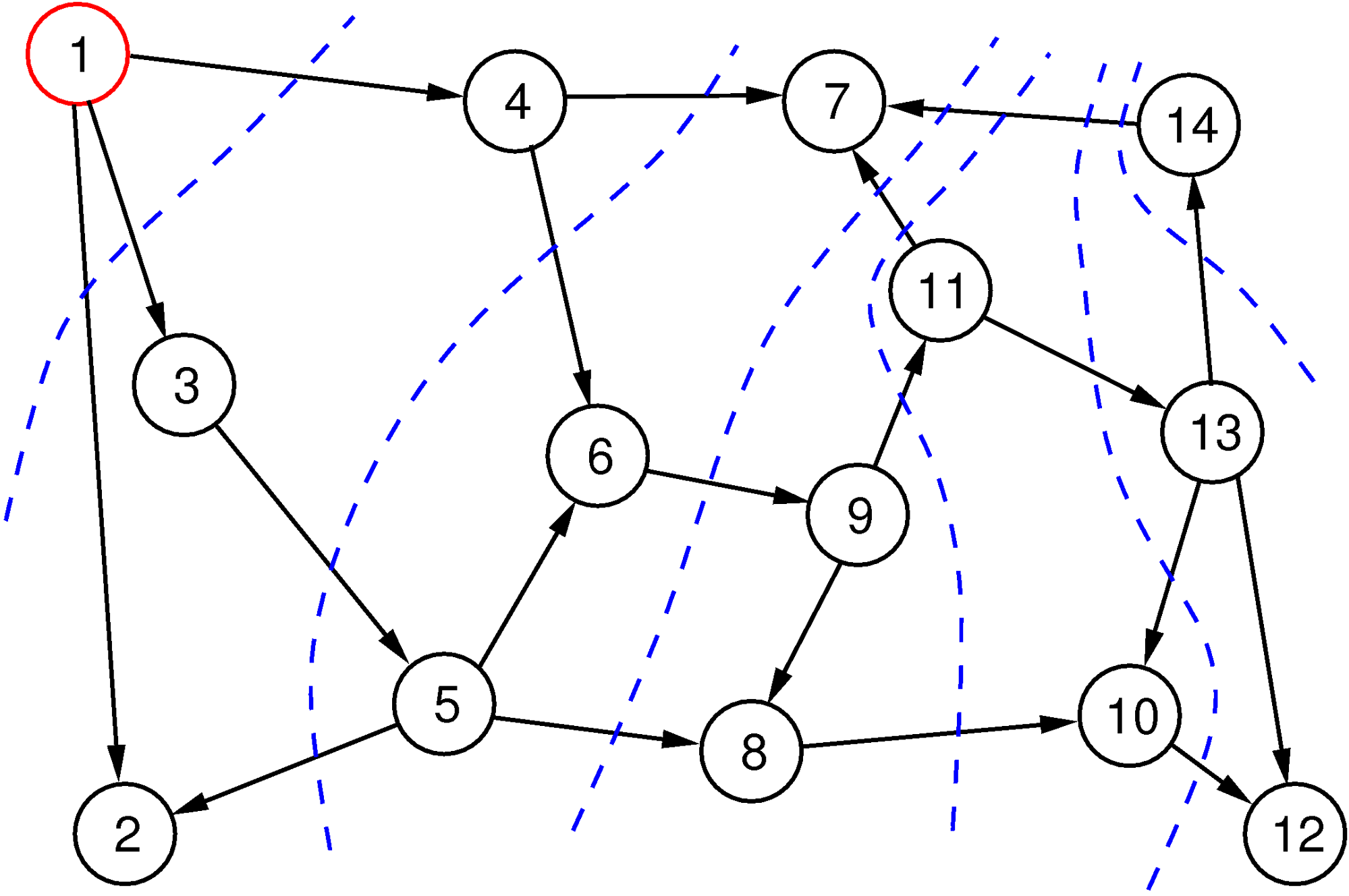
The breadth-first search method is illustrated in Figure 3. The red vertex is the start vertex, we are following edges only in the forward direction, and the numbers in the vertices tell us the order in which the vertices are visited. Layers are indicated with blue broken lines. Note that the order in which the direct neighbors are explored is arbitrary, and this choice can lead to a different order, but the layers in the various depths will always contain the same sets of vertices. Breadth-first search guarantees that it finds the shortest path from the starting vertex to all vertices.

Depth-first search uses a different strategy: it first tries to follow edges on a path as far as it gets (with a possible limitation of the depth) without going in circles. When it cannot go any further, it backtracks on its current path until it reaches a vertex from which it can follow an edge to a new vertex and goes “deep” again from there.

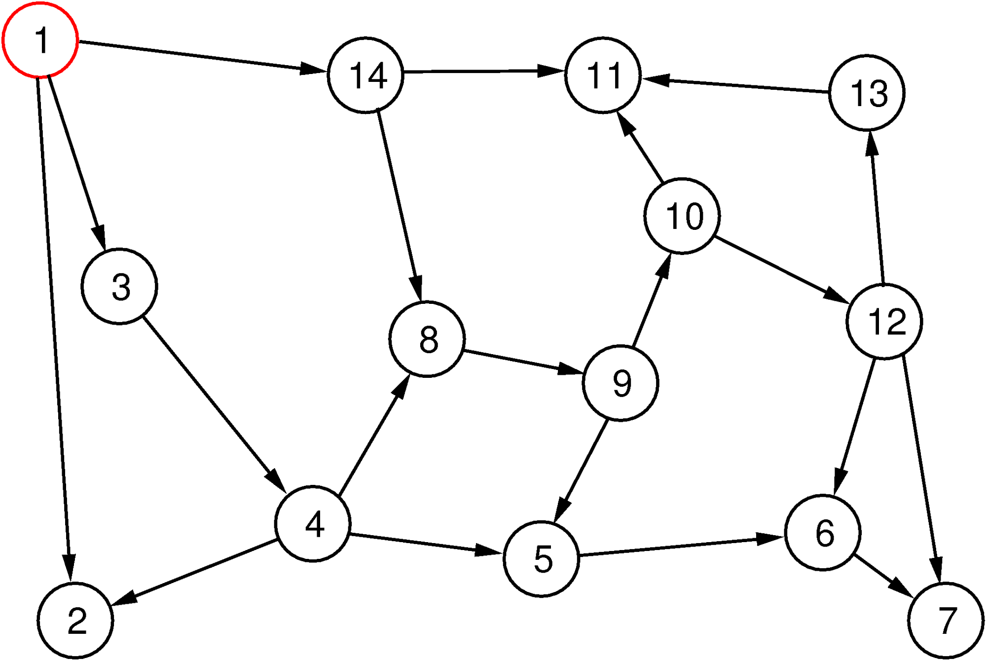
The depth-first search method is illustrated in Figure 4. The sequence of vertices visited is depicted as above, but this time there are no layers.

There are obvious variants of dealing with undirected edges or the case in which one wants to follow the edges in the backward direction or a mixture of directions, but the basic approach is the same. All of these methods are subsumed under the concept “graph traversal.”

Both methods share the same three practical challenges:

1. The crucial operation that is needed is to find the neighbors of a vertex quickly. If a vertex has k outgoing edges, we need to find the edges and the vertices on the other side of them in time O(k)—that is, in time proportional to the number.
2. Both computations can relatively quickly get out of hand since, depending on the connectivity of the graph, the number of vertices in the various layers can grow exponentially with the depth.
3. If the graph data is distributed across multiple machines (sharding), then these algorithms need a lot of network communication to do their work. Note that a network hop (around 300 microseconds) is considerably more expensive than a local lookup of data (100 nanoseconds). That is, without much care, the communication costs exceed the actual traversal costs by a large factor.

In summary, questions like “find the shortest path from A to B in a graph” use variants of Dijkstra’s algorithm, which essentially does breadth-first searches from both sides concurrently.

Graph databases

The general idea of a graph database is to store graphs and to perform graph queries on them efficiently. So, apart from the usual capability of persisting the data in a durable way and changing them with transactional workloads, they are good at answering questions about the stored graphs. Many products concentrate on doing graph queries of the above-mentioned Categories 1 (fixed path length) and 2 (local), but increasingly, capabilities in Category 3 (global) are added as well.

Note in particular that although graph databases are usually designed to excel at Category 2 problems (“local” with no a priori known path length) and generally implement graph traversal methods for this, a graph database can, in principle, equally well solve Category 1 problems by essentially using the graph infrastructure to find neighbors efficiently.

Interestingly, classical relational databases can store graphs as well in tables and are quite good in solving Category 1 problems because they only need a fixed number of join operations. However, they fail spectacularly at Category 2 problems, basically because of the a priori unknown path length.

Category 3 problems (“global”) need completely different algorithms (see, for example, Google’s Pregel framework), which we shall not discuss here in any detail.

Amongst the graph databases, there are two main groups: those using the property graph model and those using the Resource Description Framework (RDF).

A property graph is essentially a graph as described before, with the addition of “properties” for each vertex and each edge. The properties are simple key/value pairs. So, for example, each edge could have a property with a key type, and possible values could be follows or likes, or whatever. Or a vertex could have a property with a key of birthday and a timestamp as value. It is not necessary that all vertices or all edges have the same set of properties.

Contrary to that, in the Resource Description Framework, one only deals with “triples,” which consist of a subject, a predicate, and an object. A triple is essentially an edge pointing from the subject to the object with a label that is the predicate. The vertices in the graph consist of the union of the set of all subjects and the set of all objects. Potential further data associated with vertices or edges must all be modeled by additional triples. The Resource Description Framework is well standardized and is used in the Semantic Web. Data stores concentrating on RDF data are called “triple stores” and essentially implement answering SPARQL queries, which are the standard for querying RDF data. Internally, they use a variant of the graph traversal algorithm.

For any graph application but RDF, data stores using the property graph model are much more popular because most use cases can be more easily mapped onto this model, and most queries needed in practice run more efficiently, simply because a triple store would have to traverse more edges for the same query. This is why we concentrate on graph databases using the property graph model in this article.

To summarize, graph databases persist graphs, allow transactional updates to them, and are particularly good at the following classes of queries:

• enumerating the vicinity of a given vertex
• finding something in the vicinity of a given vertex
• path pattern matching
• finding the shortest paths

If done properly, a graph database also handles Category 1 queries with a fixed path length efficiently, and, increasingly, graph databases also implement Category 3 “global” queries, usually by implementing Google’s Pregel Framework, although analytics engines like Spark/GraphX are particularly good at these.

The emergence of multi-model databases

Before we consider concrete use cases for our approach, I’ll follow a little detour by explaining the idea of a multi-model database, which is getting increasingly popular these days.

We have discussed the defining characteristics and capabilities of a graph database. It turns out that, particularly for the case of property graphs, these can conveniently be combined with those of a JSON document store. The idea is that every vertex and every edge in a graph is represented by a JSON document, and every edge has two attributes denoting the unique ID of the vertex where the edge originates and where the vertex is pointing. As explained earlier, the crucial operation is to find the outgoing and incoming edges of a vertex quickly. This can be achieved with the best possible complexity by a specialized index on the edge collections. This allows implementing all of the above graph algorithms very efficiently.

Since a JSON document store is a key/value store, and in the absence of secondary indexes it can be used in a scalable way as a secondary index as well, we can conclude that the following is a viable and practical definition:

A native multi-model database is a document store, a graph database, and a key/value store all in one engine, with a common query language that supports document queries, join operations, key/value lookups, and graph queries.

The arguments above show it is feasible to build a multi-model database in this sense by using JSON documents, a specialized edge index, and a query engine that has algorithms for queries using any of the three data models, and indeed arbitrary combinations of them.

If one observes recent developments in the database market, one finds two striking facts: firstly, well-established databases that have traditionally employed a single data model add other data models and thus move toward the multi-model idea. Secondly, “native” multi-model databases emerge, which have built in this particular combination of data models from the get go.

Examples for the first observation are PostgreSQL, which added columns containing JSON data; Cassandra/DataStax, which added graph capabilities; MongoDB, which added some graph lookup facilities; and others.

Examples for the second are ArangoDB and MarkLogic. Note that MarkLogic uses an RDF triple store for its graph capabilities.

I’ll end our little deviation here with the remark that the multi-model idea allows generalizing the approach presented in this article beyond mere graph data. The basic argument remains that a multi-model database can execute smaller ad-hoc queries much more quickly than a streaming engine like Spark, which is optimized for large analytical workloads.

Multi-model graph databases at work: Concrete use cases

In this section, I’ll come back to the concrete graph data examples listed in the beginning and present a few concrete use cases for smaller ad-hoc queries.

In a social network, one is often interested in the friends of a single person, or the friends of the friends, for example, to suggest to the user somebody with similar hobbies who is not a direct friend but one with a common friend. Such information could, for example, be interesting for a real-time information service about a particular person. Other applications are to find a relatively close person with a certain property. All of these come down to a local graph traversal.

Imagine a dependency chain graph of tasks, for example. If one task is delayed, one needs to identify tasks that depend on the given task and that have an early deadline, because these are needed to judge the consequences of the delay. This is again a local graph traversal, this time with an a priori unknown path length of the result. In the other direction, one would like to see the list of those tasks on which a given task depends recursively. This is a graph traversal enumerating the vicinity of a given vertex. Both of these questions arise in real-time systems that display information about the dependency graph, and it is conceivable that a large number of users want to display such information about different parts of the graph concurrently, which leads to many small ad-hoc queries.

Next, assume a graph modeling the citations between publications—that is, a graph in which the vertices are granted patents and there is an edge from patent A to patent B if A cites B. Here, one regularly is interested in the recursive citations of a single patent, which amounts to a graph traversal. Or one looks at patent A and seeks similar patents. A good way to do this is to look at patent C that cites a patent B that A cites. This is a path pattern matching problem for paths of length 2 (one forward and one backward step). Or one would like to see all patents that recursively cite a given patent and search amongst those for a certain keyword. A need for all of these occurs in systems that allow one to browse the patent graph and retrieve “interesting” patents.

In hierarchical data—for example, a graph describing an organization, in which the people are vertices and there is an edge from the line manager of each person pointing to the person—the following questions arise naturally:

• Given a person, find the first ancestor who has access to a certain resource.
• Find all descendants of one person in a hierarchy.
• Search all descendants to find one with a particular skill.

All of these require graph traversals. Often, permission management in organizations leads to a lot of queries of similar type because, usually, the line manager of a person has all the permissions of that person as well. Therefore, finding out whether somebody has a certain permission amounts to a search for that permission amongst its descendants.

Note that all these examples are questions from Categories 1 and 2 since we are talking about relatively short, local queries. The main thesis of this article is that it makes sense to extract graph data from a graph analytics system like Hadoop/Spark into a graph database (or more generally, graph or JSON data into a multi-model database) to gain the capabilities to execute a lot of local and ad-hoc queries with very low latency.

Practicalities of multi-model databases

We have so far explored the nature of these local ad-hoc queries and considered examples of use cases in which these arise. We now turn to the practicalities and how, with today’s technology, this is actually relatively easy to achieve. For this part, I’ll use the example of ArangoDB, first of all because it is, as a native multi-model database, a full-featured graph database; and, secondly, it has the necessary deployment possibilities and import capabilities to make our approach feasible and cost efficient.

Essentially, one has to follow a simple three-step plan:

1. Deploy an ArangoDB cluster.
2. Import the data or a subset thereof, which typically resides in Hadoop.
3. Fire off ad-hoc queries.

Deployment of ArangoDB

Traditionally, deployment of distributed systems has been cumbersome, to say the least. With the advent of cloud orchestration frameworks like Apache Mesos, DC/OS, Kubernetes, and Docker Swarm, this has become much simpler. And since many do not want to use such a framework, manufacturers of distributed systems are driven toward providing a smooth user experience even without orchestration.

Provided you have a compute cluster with Apache Mesos (or Mesosphere’s DC/OS) or with Kubernetes up and running, deploying an ArangoDB cluster in there is literally a matter of issuing one command. For example:

dcos package install --options=arangodb.json arangodb3

For DC/OS (arangodb.json is a configuration file, it can be omitted to use defaults), or using the graphical UI to conjure ArangoDB up from the “Universe” repository DC/OS offers with a few mouse clicks. You can then scale your ArangoDB cluster up and down as needed from the ArangoDB UI. The orchestration framework will schedule and deploy instances within your cluster automatically and will make the best use of your compute resources. The experience for Kubernetes is very similar.

Without such an orchestration framework, let’s assume you have a compute cluster up and running with some version of Linux, Windows, or Mac OS X installed. Then deployment is as simple as downloading ArangoDB and issuing one command on the first server in an empty directory:

arangodb

Then, for each additional machine to be used, you simply issue:

arangodb --starter.join host1

Where host1 is the name or address of the first machine. Everything else is automatic, and you can easily add further machines later on in the same way.

If you have not yet deployed a compute cluster, you can set up one on a public cloud like AWS in a matter of minutes, simply using a standard Linux image. ArangoDB can be run completely using Docker containers, so deployment as described above can be done with slightly longer commands using Docker and no prior software installation step.

In any case, the details do not matter here, the main point is that it is dead simple to get started, wherever you are.

Import of the data

In most cases, your data will already reside in a Hadoop cluster stored in the Hadoop File System (HDFS). It mostly comes in the form of tabular data (comma separated values (CSV) or similar) or of document data. HDFS has a public HTTP API, and it is thus very easy to access your data from arbitrary places in your compute infrastructure, which is, of course, one of the big selling points of HDFS.

ArangoDB has an import tool called arangoimp. It can read various formats (amongst them CSV and variants as well as JSONL—one JSON document per input line) and uses batched and multi-threaded import.

To give you an idea, this is a command that imports the vertices of a patent graph into an ArangoDB cluster running one node on the local machine:

arangoimp --collection patents --file patents_arangodb.csv --type csv \
          --server.endpoint tcp://localhost:8529

It assumes that the ArangoDB is locally installed, but this command can just as easily be run from a Docker image, removing the need to install anything on your system.

Note that the patent data I used for this example can be downloaded from the Stanford Large Network Dataset Collection.

Import is fast: you can import gigabytes of data within minutes. Again, the details of the necessary steps do not matter, the main point is that data import is not a roadblock, but rather simple and swift.

Ad hoc queries

From the moment you have the data in ArangoDB you can immediately issue ad-hoc queries. Just to give you an idea, here is the above-mentioned search for similar patents, which takes a given patent, looks up its citations, and then finds all patents that also cite those:

FOR v IN 1..1 OUTBOUND "patents/6009503" GRAPH "G"
  FOR w IN 1..1 INBOUND v._id GRAPH "G"
    FILTER w._id != v._id
    RETURN w

This is ArangoDB’s own query language AQL, which can be used from any language driver in exactly the same way. It allows performing graph queries, document queries, and key lookups, all in one language. In the graph domain, it covers all three categories: constant path length queries; local queries with variable path length; and Pregel-type global queries, which are run in a distributed fashion across the ArangoDB cluster.

As another example, to count all recursively cited patents from one given patent up to depth 10 one would do this:

FOR v IN 1..10 OUTBOUND "patents/3541687" GRAPH "G"
  COLLECT WITH COUNT INTO c
  RETURN c

Execution times for such queries are between 1 milliseconds and some dozens of milliseconds, depending on the graph and the size of the graph traversal being performed.

Conclusion

To summarize, in this article we have discussed various types of graph queries, have considered the concept of the graph traversal class of algorithms, and have explored the idea that one can get greater value out of available graph data by importing it into a specialized graph database to tap into its capabilities to do local ad-hoc queries and thus considerably enhance and extend the analyst’s arsenal.

As an aside, the multi-model idea broadens the scope of this approach beyond mere graph applications and well into data analysis tools on arbitrary JSON data.

Furthermore, I’ve shown that implementing this idea is not a scary and difficult task, but rather convenient, straightforward, and quick with today’s deployment tools.

(See my talk at Dataworks Summit 2017 in Munich to learn more about the topic of this article.)