Introduction to LSTMs with TensorFlow
How to build a multilayered LSTM network to infer stock market sentiment from social conversation using TensorFlow.
 Network (source: Pixabay)
Long short-term memory (LSTM) networks have been around for 20 years (Hochreiter and Schmidhuber, 1997), but have seen a tremendous growth in popularity and success over the last few years. LSTM networks are a specialized type of recurrent neural network (RNN)—a neural network architecture used for modeling sequential data and often applied to natural language processing (NLP) tasks. The advantage of LSTMs over traditional RNNs is that they retain information for long periods of time, allowing for important information learned early in the sequence to have a larger impact on model decisions made at the end of the sequence.
In this tutorial, we will introduce the LSTM network architecture and build our own LSTM network to classify stock market sentiment from messages on StockTwits. We use TensorFlow because it offers compact, high-level commands and is very popular these days.

Learn faster. Dig deeper. See farther.
LSTM cells and network architecture
Before we dive into building our network, let’s go through a brief introduction of how LSTM cells work and an LSTM network architecture (Figure 1).
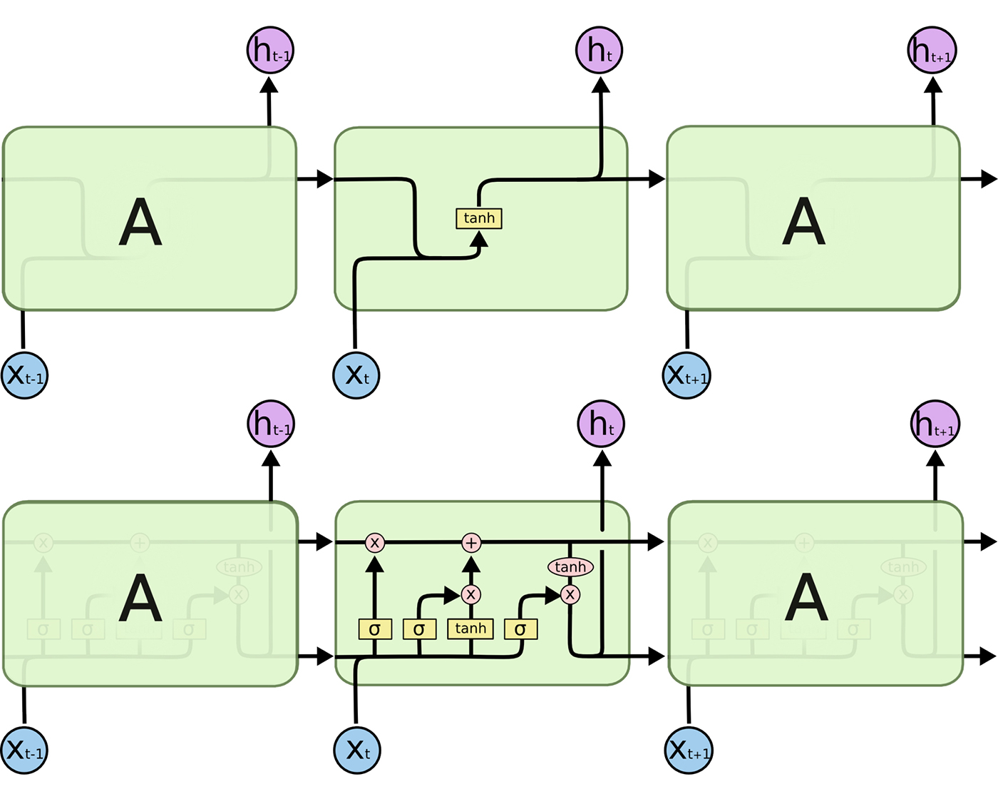
\(A\) represents a full RNN cell that takes the current input of the sequence (in our case the current word), \(x_i\), and outputs the current hidden state, \(h_i\), passing this to the next RNN cell for our input sequence. The inside of a LSTM cell is a lot more complicated than a traditional RNN cell. While the traditional RNN cell has a single “internal layer” acting on the current state \((h_{t-1})\) and input \((x_t)\), the LSTM cell has three.
First we have the “forget gate” that controls what information is maintained from the previous state. This takes in the previous cell output \(h_{t-1}\) and the current input \(x_t\) band applies a sigmoid activation layer \((\sigma)\) to get values between 0 and 1 for each hidden unit. This is followed by element-wise multiplication with the current state (the first operation in the “upper conveyor belt” in Figure 1).
Next is an “update gate” that updates the state based on the current input. This passes the same input (\(h_{t-1}\) and \(x_t\)) into a sigmoid activation layer \((\sigma)\) and into a tanh activation layer \((tanh)\) and performs element-wise multiplication between these two results. Next, element-wise addition is performed with the result and the current state after applying the “forget gate” to update the state with new information. (The second operation in the “upper conveyor belt” in Figure 1.)
Finally, we have an “output gate” that controls what information gets passed to the next state. We run the current state through a tanh activation layer \((tanh)\) and perform element-wise multiplication with the cell input (\(h_{t-1}\) and \(x_t\)) run through a sigmoid layer \((\sigma)\) that acts as a filter on what we decide to output. This output \(h_t\) is then passed to the LSTM cell for the next input of our sequence and also passed up to the next layer of our network.
Now that we have a better understanding of an LSTM cell, let’s look at an example LSTM network architecture in Figure 2.
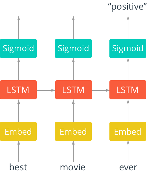
In Figure 2, we see an “unrolled” LSTM network with an embedding layer, a subsequent LSTM later, and a sigmoid activation function. We see that our inputs, in this case words in a movie review, are input sequentially.
The words are first input into an embedding lookup. In most cases, when working with a corpus of text data, the size of the vocabulary is particularly large. Because of this, it is often beneficial (in terms of accuracy and efficiency) to use a word embedding. This is a multidimensional, distributed representation of words in a vector space. These embeddings can be learned using other deep learning techniques like word2vec or, as we will do here, we can train the model in an end-to-end fashion to learn the embeddings as we train.
These embeddings are then input into our LSTM layer, where the output is fed to a sigmoid output layer and the LSTM cell for the next word in our sequence. In our case, we care only about the model output after the entire sequence has been evaluated, so we consider only the output of the sigmoid activation layer for the final word in our sequence.
Setup
You can access the code for this tutorial on GitHub. All instructions are in the README file in the repository.
StockTwits $SPY message data set
We are going to train our LSTM to predict the sentiment of an individual based on a comment made about the stock market.
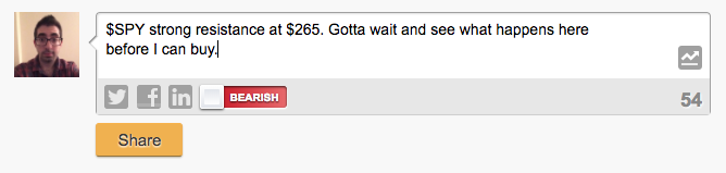
We will train the model using messages tagged with $SPY, the S&P 500 index fund, from StockTwits.com. StockTwits is a social media network for traders and investors to share their views about the stock market. When a user posts a message, they tag the relevant stock ticker ($SPY, in our case) and have the option to tag the messages with their sentiment—“bullish” if they believe the stock will go up and “bearish” if they believe the stock will go down. Figure 3 shows a sample message.
Our data set consists of approximately 100,000 messages posted in 2017 that are tagged with $SPY where the user indicated their sentiment.
Processing data for modeling
Before we get into the modeling, we have to do a bit of processing on our data. The GitHub repository includes a utils module that has the code for preprocessing and batching our data. These functions abstract away a lot of the data work for our tutorial. But please read through the “util.py” file to get a better understanding of how to preprocess the data for analysis.
First, we need to preprocess the messages data to normalize for known StockTwits entities, such as a reference to a ticker symbol, a user, a link, or a reference to a number. Here, we also remove punctuation.
Next, we encode our message and sentiment data. The sentiment is simply encoded as a 0 for bearish message and a 1 for a bullish message. To encode our message data, first we collect our full vocabulary across all messages and map each word to a unique index, starting with 1. Note that in practice you will want to use only the vocabulary from the training data, but for simplicity and demonstration purposes, we will create the vocabulary from our entire data set. Once we have this mapping, we replace each word in each message with its appropriate index.
We want all of our data inputs to be of equal size, so we need to find the maximum sequence length and then zero pad our data. Here, we make all message sequences the maximum length (in our case 244 words) and “left pad” shorter messages with 0s.
Finally, we split our data set into train, validation, and test sets for modeling.
Network inputs
The first thing we do when building a neural network is define our network inputs. Here, we simply define a function to build TensorFlow placeholders for our message sequences, our labels, and a variable called “keep probability” associated with dropout (we will talk more about this later).
defmodel_inputs():"""Create the model inputs"""inputs_=tf.placeholder(tf.int32,[None,None],name='inputs')labels_=tf.placeholder(tf.int32,[None,None],name='labels')keep_prob_=tf.placeholder(tf.float32,name='keep_prob')
TensorFlow placeholders are simply “pipes” for data that we will feed into our network during training.
Embedding layer
Next, we define a function to build our embedding layer. In TensorFlow, the word embeddings are represented as a matrix whose rows are the vocabulary and the columns are the embeddings (see Figure 4). Each value is a weight that will be learned during our training process.
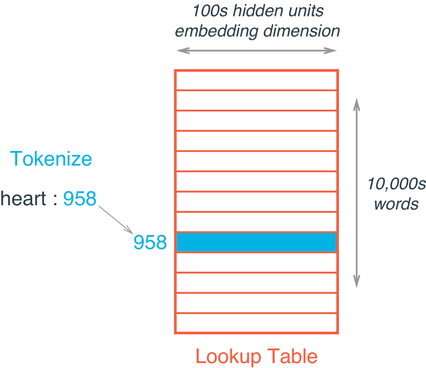
The embedding lookup is then just a simple lookup from our embedding matrix based on the index of the current word.
defbuild_embedding_layer(inputs_,vocab_size,embed_size):"""Create the embedding layer"""embedding=tf.Variable(tf.random_uniform((vocab_size,embed_size),-1,1))embed=tf.nn.embedding_lookup(embedding,inputs_)
The resulting word embedding vector is our distributed representation—i.e., multi-dimensional vector, of the current word that will be passed to the LSTM layers.
LSTM Layers
We will set up a function to build the LSTM Layers to dynamically handle the number of layers and sizes. The function will take a list of LSTM sizes, which will also indicate the number of LSTM layers based on the list’s length (e.g., our example will use a list of length 2, containing the sizes 128 and 64, indicating a two-layered LSTM network where the first layer has hidden layer size 128 and the second layer has hidden layer size 64).
First, we build our LSTM layers using the TensorFlow contrib API’s BasicLSTMCell and wrapping each layer in a dropout layer.
Note that we will use the BasicLSTMCell here for illustrative purposes only. There are more performant ways to define our network in production, such as the tf.contrib.cudnn_rnn.CudnnCompatibleLSTMCell, which is 20x faster than the BasicLSTMCell and uses 3-4x less memory.
Dropout is a regularization technique used in deep learning, where any individual node has a probability of “dropping out” of the network during a given iteration of learning. It is a good practice to use these regularizations when tackling real-world problems. These techniques make the model more generalizable to unseen data by ensuring that the model is not too dependent on any given node.
defbuild_lstm_layers(lstm_sizes,embed,keep_prob_,batch_size):"""Create the LSTM layers"""lstms=[tf.contrib.rnn.BasicLSTMCell(size)forsizeinlstm_sizes]# Add dropout to the celldrops=[tf.contrib.rnn.DropoutWrapper(lstm,output_keep_prob=keep_prob_)forlstminlstms]# Stack up multiple LSTM layers, for deep learningcell=tf.contrib.rnn.MultiRNNCell(drops)# Getting an initial state of all zerosinitial_state=cell.zero_state(batch_size,tf.float32)lstm_outputs,final_state=tf.nn.dynamic_rnn(cell,embed,initial_state=initial_state)
This list of dropout wrapped LSTMs are then passed to a TensorFlow MultiRNN cell to stack the layers together. Finally, we create an initial zero state and pass our stacked LSTM layers, our input from the embedding layer we defined previously, and the initial state to create the network. The Tensorflow dynamic_rnn call returns the model output and the final state, which we will need to pass between batches while training.
Loss function, optimizer, and accuracy
Finally, we create functions to define our model loss function, our optimizer, and our accuracy. Even though the loss and accuracy are just calculations based on results, everything in TensorFlow is part of a computation graph. Therefore, we need to define our loss, optimizer, and accuracy nodes in the context of our graph.
defbuild_cost_fn_and_opt(lstm_outputs,labels_,learning_rate):"""Create the Loss function and Optimizer"""predictions=tf.contrib.layers.fully_connected(lstm_outputs[:,-1],1,activation_fn=tf.sigmoid)loss=tf.losses.mean_squared_error(labels_,predictions)optimzer=tf.train.AdadeltaOptimizer(learning_rate).minimize(loss)defbuild_accuracy(predictions,labels_):"""Create accuracy"""correct_pred=tf.equal(tf.cast(tf.round(predictions),tf.int32),labels_)accuracy=tf.reduce_mean(tf.cast(correct_pred,tf.float32))
First, we get our predictions by passing the final output of the LSTM layers to a sigmoid activation function via a TensorFlow fully connected layer. Recall that the LSTM layer outputs a result for all of the words in our sequence. However, we want only the final output for making predictions. We pull this out using the [: , -1] indexing demonstrated above, and pass this through a single fully connected layer with sigmoid activation to get our predictions. These predictions are fed to our mean squared error loss function and use the Adadelta optimizer to minimize the loss. Finally, we define our accuracy metric for assessing the model performance across our training, validation, and test sets.
Building the graph and training
Now that we have defined functions to create the pieces of our computational graph, we define one more function that will build the computational graph and train the model. First, we call each of the functions we have defined to construct the network and call a TensorFlow session to train the model over a predefined number of epochs using mini-batches. At the end of each epoch, we will print the loss, training accuracy, and validation accuracy to monitor the results as we train.
defbuild_and_train_network(lstm_sizes,vocab_size,embed_size,epochs,batch_size,learning_rate,keep_prob,train_x,val_x,train_y,val_y):# Build Graphwithtf.Session()assess:# Train Network# Save Network
Next, we define our model hyperparameters. We will build a two-layer LSTM network with hidden layer sizes of 128 and 64, respectively. We will use an embedding size of 300 and train over 50 epochs with mini-batches of size 256. We will use an initial learning rate of 0.1, though our Adadelta optimizer will adapt this over time, and a keep probability of 0.5.
Output shows that our LSTM network starts to learn rather quickly, jumping from 58% validation accuracy after the first epoch to 66% validation accuracy after the 10th. Learning then begins to slow down, ultimately reaching a training accuracy of 75% and validation accuracy of 72% after just 50 epochs of training. When the model is done training, we use a TensorFlow saver to save out model parameters for later use.
Epoch:1/50...Batch:303/303...TrainLoss:0.247...TrainAccuracy:0.562...ValAccuracy:0.578Epoch:2/50...Batch:303/303...TrainLoss:0.245...TrainAccuracy:0.583...ValAccuracy:0.596Epoch:3/50...Batch:303/303...TrainLoss:0.247...TrainAccuracy:0.597...ValAccuracy:0.617Epoch:4/50...Batch:303/303...TrainLoss:0.240...TrainAccuracy:0.610...ValAccuracy:0.627Epoch:5/50...Batch:303/303...TrainLoss:0.238...TrainAccuracy:0.620...ValAccuracy:0.632Epoch:6/50...Batch:303/303...TrainLoss:0.234...TrainAccuracy:0.632...ValAccuracy:0.642Epoch:7/50...Batch:303/303...TrainLoss:0.230...TrainAccuracy:0.636...ValAccuracy:0.648Epoch:8/50...Batch:303/303...TrainLoss:0.227...TrainAccuracy:0.641...ValAccuracy:0.653Epoch:9/50...Batch:303/303...TrainLoss:0.223...TrainAccuracy:0.646...ValAccuracy:0.656Epoch:10/50...Batch:303/303...TrainLoss:0.221...TrainAccuracy:0.652...ValAccuracy:0.659
Testing
Finally, we check our model results on the test set to make sure they are in line with what we expect based on the validation set we observed during training.
deftest_network(model_dir,batch_size,test_x,test_y):# Build Networkwithtf.Session()assess:# Restore Model# Test Model
We build the computational graph just like we did before, but now instead of training we restore our saved model from our checkpoint directory and then run our test data through the model. The test accuracy is 72%. This is right in line with our validation accuracy and indicates that we captured an appropriate distribution of our data across our data split.
INFO:tensorflow:Restoringparametersfromcheckpoints/sentiment.ckptTestAccuracy:0.717
Conclusion
We are off to a great start, but from here we can do a few things to improve model performance. We can train the model longer, build a larger network with more hidden units and more LSTM layers, and tune our hyperparameters.
In summary, LSTM networks are an extension of RNNs that are designed to handle the problem of learning long-term dependencies. LSTMs have broad-reaching applications when dealing with sequential data and are often used for NLP tasks. We have demonstrated the expressive power of LSTMs by training a multilayered LSTM network with word embeddings to model stock market sentiment from comments made on social media.
This post is a collaboration between O’Reilly and TensorFlow. See our statement of editorial independence.