Reinforcement learning with TensorFlow
Solving problems with gradient ascent, and training an agent in Doom.
 Mountain climbing (source: Pixabay)
The world of deep reinforcement learning can be a difficult one to grasp. Between the sheer number of acronyms and learning models, it can be hard to figure out the best approach to take when trying to learn how to solve a reinforcement learning problem. Reinforcement learning theory is not something new; in fact, some aspects of reinforcement learning date back to the mid-1950s. If you are absolutely fresh to reinforcement learning, I suggest you check out my previous article, “Introduction to reinforcement learning and OpenAI Gym,” to learn the basics of reinforcement learning.
Deep reinforcement learning requires updating large numbers of gradients, and deep learning tools such as TensorFlow are extremely useful for calculating these gradients. Deep reinforcement learning also requires visual states to be represented abstractly, and for this, convolutional neural networks work best. In this article, we will use Python, TensorFlow, and the reinforcement learning library Gym to solve the 3D Doom health gathering environment. For a full version of the code and required dependencies, please access the GitHub repository and Jupyter Notebook for this article.

Learn faster. Dig deeper. See farther.
Exploring the environment
In this environment, the Doom player is standing on top of acid water and needs to learn how to navigate and collect health packs to stay alive.
One method of reinforcement learning we can use to solve this problem is the REINFORCE with baselines algorithm. Reinforce is very simple—the only data it needs includes states and rewards from an environment episode. Reinforce is called a policy gradient method because it solely evaluates and updates an agent’s policy. A policy is the way the agent will behave in a current state. For example, in the game pong, a simple policy would be: if the ball is moving at a certain angle, the best action would be to move the paddle to a position relative to that angle. On top of using a convolutional neural network to estimate the best policy for any given state, we will use the same network to estimate the value or predicted long-term reward at a given state.
We will start by defining our environment using Gym.
env=gym.make('ppaquette/DoomHealthGathering-v0')
Before trying to get an agent to learn, let’s look at a standard baseline of observing a random agent. It’s clear to see we have a lot to learn.
Setting up our learning environment
Reinforce is considered a Monte Carlo method of learning, this means that the agent will collect data from an entire episode then perform calculations at the end of that episode. In our case, we will gather a batch of multiple episodes to train on. We will set up our environment training data as empty lists, which we will append our data into for each step.
states,actions,rewards=[],[],[]
We next define some of our hyper parameters that our neural network will use.
# Hyper Parametersalpha=1e-4gamma=0.99
Alpha is our usual learning rate, and gamma is our rate of reward discounting. Reward discounting is a way of evaluating potential future rewards given the reward history from an agent. As the discount rate approaches zero, the agent is only concerned with immediate rewards and does not consider potential future rewards. We can write a simple function to evaluate a set of rewards from an episode, with the following:
defdiscount(r,gamma,normal):discount=np.zeros_like(r)G=0.0foriinreversed(range(0,len(r))):G=G*gamma+r[i]discount[i]=G# Normalizeifnormal:mean=np.mean(discount)std=np.std(discount)discount=(discount-mean)/(std)returndiscount
Let’s evaluate the following sets of rewards:
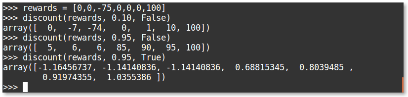
You can see that with the high discounting, the large negative reward in the middle is slightly disregarded due to the large reward at the end. We can also add normalization to our discounted rewards to make sure the reward range stays small; this was extremely important for being able to solve the doom environment.
Our value function will constantly be trying to approximate the discounted reward for any given state.
Building the convolutional neural network
Next, we will build our convolutional neural network for taking in a state and outputting action probabilities and state values. We will have three actions to choose from: move forward, move right, and move left. The policy approximation is setup exactly the same as an image classifier, but instead of the outputs representing the confidence of a class, our outputs will represent our confidence in taking a certain action. Compared to large image classification models, when it comes to reinforcement learning, simple networks work best.
We will use a convnet similar to what was used for the famous DQN algorithm. Our network will input a processed resized image of 84×84 pixels, output 16 convolutions of a 8×8 kernel with a stride of 4, followed by 32 convolutions with a 8×8 kernel and a stride of 4, finished with a fully connected layer of 256 neurons. For the convolutional layers, we will use VALID padding, which will shrink the image quite aggressively.
Both our policy approximation and our value approximation will share the same convolutional neural network to calculate their values.
# Conv Layersconvs=[16,32]kerns=[8,8]strides=[4,4]pads='valid'fc=256activ=tf.nn.elu# Policy Networkconv1=tf.layers.conv2d(inputs=X,filters=convs[0],kernel_size=kerns[0],strides=strides[0],padding=pads,activation=activ,name='conv1')conv2=tf.layers.conv2d(inputs=conv1,filters=convs[1],kernel_size=kerns[1],strides=strides[1],padding=pads,activation=activ,name='conv2')flat=tf.layers.flatten(conv2)dense=tf.layers.dense(inputs=flat,units=fc,activation=activ,name='fc')logits=tf.layers.dense(inputs=dense,units=n_actions,name='logits')value=tf.layers.dense(inputs=dense,units=1,name='value')calc_action=tf.multinomial(logits,1)aprob=tf.nn.softmax(logits)action_logprob=tf.nn.log_softmax(logits)
In deep learning, weight initialization is extremely important, by default tf.layers will initialize the weights using the glorot uniform initializer also known as xavier initialization. If you initialize the weights with too large of a deviation, the agent will act biased, too small and the agent will act extremely randomly. Ideally, the agent will first begin acting mainly random, then will slowly change the weight values to maximize reward. In reinforcement learning, this is known as exploration versus exploitation because initially the agent will act randomly exploring the environment, and with each update it will move its action probabilities slightly toward actions that receive good rewards.
Measuring and increasing performance
So now that we have the model built, how are we going to have it learn? The solution is elegantly simple. We want to change the network’s weights so it will increase its confidence in what action to take, and the amount of change is based upon our baseline of how accurate our value estimation was. Overall, we need to minimize our total loss.
Implementing this in TensorFlow, we measure our policy loss by using the sparse_softmax_cross_entropy function. The sparse means that our action labels are single integers and the logits are our final unactivated policy output. This function calculates the softmax and log loss for us. As confidence in a taken action approaches 1, the loss approaches 0.
We then multiply the cross entropy loss by the difference of our discounted reward and our value approximation. We calculate our value loss by using the common squared mean error loss. We then add our losses together to calculate our total loss.
# Define Lossespg_loss=tf.reduce_mean((D_R-value)*tf.nn.sparse_softmax_cross_entropy_with_logits(logits=logits,labels=Y))value_loss=value_scale*tf.reduce_mean(tf.square(D_R-value))entropy_loss=-entropy_scale*tf.reduce_sum(aprob*tf.exp(aprob))loss=pg_loss+value_loss-entropy_loss# Create Optimizeroptimizer=tf.train.AdamOptimizer(alpha)grads=tf.gradients(loss,tf.trainable_variables())grads,_=tf.clip_by_global_norm(grads,gradient_clip)# gradient clippinggrads_and_vars=list(zip(grads,tf.trainable_variables()))train_op=optimizer.apply_gradients(grads_and_vars)# Initialize Sessionsess=tf.Session()init=tf.global_variables_initializer()sess.run(init)
Training the agent
We are now ready to train the agent. We feed our current state into the network and get our action by calling the tf.multinomial function. We perform that action and store the state, action, and future reward. We then store the new resized state2 as our current state and repeat this procedure until the end of the episode. We then append our state, action, and reward data into a new list, which we will use for feeding into the network, for evaluating a batch.
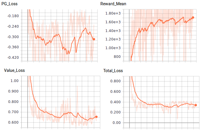
Depending on our intial weight initialization, our agent should eventually solve the environment in roughly 200 training batches with an average reward of 1,200. OpenAI’s standard for solving the environment is getting an average reward of 1,000 over 100 consecutive trials. Allowing the agent to train further, it was able to achieve an average of 1,700 but couldn’t seem to beat this average. Here is my agent after 1,000 training batches:
If you want to test your agent’s confidence at any given frame, all you need to do is feed that state into the network and observe the output. Here, while facing just the wall, the agent had 90% confidence that the best action was to turn right, and in the following picture on the right, the agent was only 61% confident that going forward was the best action.
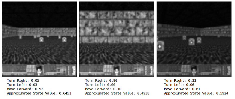
If you are keen, you may think to yourself that that 61% confidence for what seems like a clearly good move is not that great, and you would be right. I suspect our agent has mainly learned to avoid walls extremely well, and since the agent only receives rewards for surviving, it’s not exclusively trying to pick up health packs. Picking up health packs is just correlated with surviving longer. In some ways, I would not consider this agent fully intelligent. The agent also almost completely disregards turning left. The agent has a simple policy, but it has learned it on it’s own, and it works!
Moving forward
So, I hope you now understand the basics of policy gradient methods. These are the building blocks of moving forward to more advanced policy gradient methods, such as Advantage Actor-Critic methods, A3C or PPO. The Reinforce model does not take into account state transitions, action values, or the TD error. It also deals with the problem of credit assignment. To solve these issues, you need multiple neural networks and more intelligent training data. There are also many experiments one could conduct to try to improve performance; such as tweaking the hyperparameters. With some minor modification, you can use this exact same network to solve a large variety of Atari games as well. So, go forth and see just how many problems you can solve!
This post is a collaboration between O’Reilly and TensorFlow. See our statement of editorial independence.