Streaming 101: The world beyond batch
A high-level tour of modern data-processing concepts.
 Three women wading in a stream gathering leeches (source: Wellcome Library, London)
Streaming data processing is a big deal in big data these days, and for good reasons. Amongst them:
- Businesses crave ever more timely data, and switching to streaming is a good way to achieve lower latency.
- The massive, unbounded data sets that are increasingly common in modern business are more easily tamed using a system designed for such never-ending volumes of data.
- Processing data as they arrive spreads workloads out more evenly over time, yielding more consistent and predictable consumption of resources.
Despite this business-driven surge of interest in streaming, the majority of streaming systems in existence remain relatively immature compared to their batch brethren, which has resulted in a lot of exciting, active development in the space recently.

Learn faster. Dig deeper. See farther.
As someone who’s worked on massive-scale streaming systems at Google for the last five+ years (MillWheel, Cloud Dataflow), I’m delighted by this streaming zeitgeist, to say the least. I’m also interested in making sure that folks understand everything that streaming systems are capable of and how they are best put to use, particularly given the semantic gap that remains between most existing batch and streaming systems. To that end, the fine folks at O’Reilly have invited me to contribute a written rendition of my Say Goodbye to Batch talk from Strata + Hadoop World London 2015. Since I have quite a bit to cover, I’ll be splitting this across two separate posts:
- Streaming 101: This first post will cover some basic background information and clarify some terminology before diving into details about time domains and a high-level overview of common approaches to data processing, both batch and streaming.
- The Dataflow Model: The second post will consist primarily of a whirlwind tour of the unified batch + streaming model used by Cloud Dataflow, facilitated by a concrete example applied across a diverse set of use cases. After that, I’ll conclude with a brief semantic comparison of existing batch and streaming systems.
So, long-winded introductions out of the way, let’s get nerdy.
Background
To begin with, I’ll cover some important background information that will help frame the rest of the topics I want to discuss. We’ll do this in three specific sections:
- Terminology: To talk precisely about complex topics requires precise definitions of terms. For some terms that have overloaded interpretations in current use, I’ll try to nail down exactly what I mean when I say them.
- Capabilities: I’ll remark on the oft-perceived shortcomings of streaming systems. I’ll also propose the frame of mind that I believe data processing system builders need to adopt in order to address the needs of modern data consumers going forward.
- Time domains: I’ll introduce the two primary domains of time that are relevant in data processing, show how they relate, and point out some of the difficulties these two domains impose.
Terminology: What is streaming?
Before going any further, I’d like to get one thing out of the way: what is streaming? The term “streaming” is used today to mean a variety of different things (and for simplicity, I’ve been using it somewhat loosely up until now), which can lead to misunderstandings about what streaming really is, or what streaming systems are actually capable of. As such, I would prefer to define the term somewhat precisely.
The crux of the problem is that many things that ought to be described by what they are (e.g., unbounded data processing, approximate results, etc.), have come to be described colloquially by how they historically have been accomplished (i.e., via streaming execution engines). This lack of precision in terminology clouds what streaming really means, and in some cases, burdens streaming systems themselves with the implication that their capabilities are limited to characteristics frequently described as “streaming,” such as approximate or speculative results. Given that well-designed streaming systems are just as capable (technically more so) of producing correct, consistent, repeatable results as any existing batch engine, I prefer to isolate the term streaming to a very specific meaning: a type of data processing engine that is designed with infinite data sets in mind. Nothing more. (For completeness, it’s perhaps worth calling out that this definition includes both true streaming and micro-batch implementations.)
As to other common uses of “streaming,” here are a few that I hear regularly, each presented with the more precise, descriptive terms that I suggest we as a community should try to adopt:
- Unbounded data: A type of ever-growing, essentially infinite data set. These are often referred to as “streaming data.” However, the terms streaming or batch are problematic when applied to data sets, because as noted above, they imply the use of a certain type of execution engine for processing those data sets. The key distinction between the two types of data sets in question is, in reality, their finiteness, and it’s thus preferable to characterize them by terms that capture this distinction. As such, I will refer to infinite “streaming” data sets as unbounded data, and finite “batch” data sets as bounded data.
- Unbounded data processing: An ongoing mode of data processing, applied to the aforementioned type of unbounded data. As much as I personally like the use of the term streaming to describe this type of data processing, its use in this context again implies the employment of a streaming execution engine, which is at best misleading; repeated runs of batch engines have been used to process unbounded data since batch systems were first conceived (and conversely, well-designed streaming systems are more than capable of handling “batch” workloads over bounded data). As such, for the sake of clarity, I will simply refer to this as unbounded data processing.
- Low-latency, approximate, and/or speculative results: These types of results are most often associated with streaming engines. The fact that batch systems have traditionally not been designed with low-latency or speculative results in mind is a historical artifact, and nothing more. And of course, batch engines are perfectly capable of producing approximate results if instructed to. Thus, as with the terms above, it’s far better describing these results as what they are (low-latency, approximate, and/or speculative) than by how they have historically been manifested (via streaming engines).
From here on out, any time I use the term “streaming,” you can safely assume I mean an execution engine designed for unbounded data sets, and nothing more. When I mean any of the other terms above, I will explicitly say unbounded data, unbounded data processing, or low-latency / approximate / speculative results. These are the terms we’ve adopted within Cloud Dataflow, and I encourage others to take a similar stance.
On the greatly exaggerated limitations of streaming
Next up, let’s talk a bit about what streaming systems can and can’t do, with an emphasis on can; one of the biggest things I want to get across in these posts is just how capable a well-designed streaming system can be. Streaming systems have long been relegated to a somewhat niche market of providing low-latency, inaccurate/speculative results, often in conjunction with a more capable batch system to provide eventually correct results, i.e. the Lambda Architecture.
For those of you not already familiar with the Lambda Architecture, the basic idea is that you run a streaming system alongside a batch system, both performing essentially the same calculation. The streaming system gives you low-latency, inaccurate results (either because of the use of an approximation algorithm, or because the streaming system itself does not provide correctness), and some time later a batch system rolls along and provides you with correct output. Originally proposed by Twitter’s Nathan Marz (creator of Storm), it ended up being quite successful because it was, in fact, a fantastic idea for the time; streaming engines were a bit of a letdown in the correctness department, and batch engines were as inherently unwieldy as you’d expect, so Lambda gave you a way to have your proverbial cake and eat it, too. Unfortunately, maintaining a Lambda system is a hassle: you need to build, provision, and maintain two independent versions of your pipeline, and then also somehow merge the results from the two pipelines at the end.
As someone who has spent years working on a strongly-consistent streaming engine, I also found the entire principle of the Lambda Architecture a bit unsavory. Unsurprisingly, I was a huge fan of Jay Kreps’ Questioning the Lambda Architecture post when it came out. Here was one of the first highly visible statements against the necessity of dual-mode execution; delightful. Kreps addressed the issue of repeatability in the context of using a replayable system like Kafka as the streaming interconnect, and went so far as to propose the Kappa Architecture, which basically means running a single pipeline using a well-designed system that’s appropriately built for the job at hand. I’m not convinced that notion itself requires a name, but I fully support the idea in principle.
Quite honestly, I’d take things a step further. I would argue that well-designed streaming systems actually provide a strict superset of batch functionality. Modulo perhaps an efficiency delta[1], there should be no need for batch systems as they exist today. And kudos to the Flink folks for taking this idea to heart and building a system that’s all-streaming-all-the-time under the covers, even in “batch” mode; I love it.
The corollary of all this is that broad maturation of streaming systems combined with robust frameworks for unbounded data processing will, in time, allow the relegation of the Lambda Architecture to the antiquity of big data history where it belongs. I believe the time has come to make this a reality. Because to do so, i.e. to beat batch at its own game, you really only need two things:
- Correctness — This gets you parity with batch.At the core, correctness boils down to consistent storage. Streaming systems need a method for checkpointing persistent state over time (something Kreps has talked about in his Why local state is a fundamental primitive in stream processing post), and it must be well-designed enough to remain consistent in light of machine failures. When Spark Streaming first appeared in the public big data scene a few years ago, it was a beacon of consistency in an otherwise dark streaming world. Thankfully, things have improved somewhat since then, but it is remarkable how many streaming systems still try to get by without strong consistency; I seriously cannot believe that at-most-once processing is still a thing, but it is. To reiterate, because this point is important: strong consistency is required for exactly-once processing, which is required for correctness, which is a requirement for any system that’s going to have a chance at meeting or exceeding the capabilities of batch systems. Unless you just truly don’t care about your results, I implore you to shun any streaming system that doesn’t provide strongly consistent state. Batch systems don’t require you to verify ahead of time if they are capable of producing correct answers; don’t waste your time on streaming systems that can’t meet that same bar. If you’re curious to learn more about what it takes to get strong consistency in a streaming system, I recommend you check out the MillWheel and Spark Streaming papers. Both papers spend a significant amount of time discussing consistency. Given the amount of quality information on this topic in the literature and elsewhere, I won’t be covering it any further in these posts.
- Tools for reasoning about time — This gets you beyond batch.Good tools for reasoning about time are essential for dealing with unbounded, unordered data of varying event-time skew. An increasing number of modern data sets exhibit these characteristics, and existing batch systems (as well as most streaming systems) lack the necessary tools to cope with the difficulties they impose. I will spend the remainder of this post, and the bulk of the next post, explaining and focusing on this point. To begin with, we’ll get a basic understanding of the important concept of time domains, after which we’ll take a deeper look at what I mean by unbounded, unordered data of varying event-time skew. We’ll then spend the rest of this post looking at common approaches to bounded and unbounded data processing, using both batch and streaming systems.
Event time vs. processing time
To speak cogently about unbounded data processing requires a clear understanding of the domains of time involved. Within any data processing system, there are typically two domains of time we care about:
- Event time, which is the time at which events actually occurred.
- Processing time, which is the time at which events are observed in the system.
Not all use cases care about event times (and if yours doesn’t, hooray! — your life is easier), but many do. Examples include characterizing user behavior over time, most billing applications, and many types of anomaly detection, to name a few.
In an ideal world, event time and processing time would always be equal, with events being processed immediately as they occur. Reality is not so kind, however, and the skew between event time and processing time is not only non-zero, but often a highly variable function of the characteristics of the underlying input sources, execution engine, and hardware. Things that can affect the level of skew include:
- Shared resource limitations, such as network congestion, network partitions, or shared CPU in a non-dedicated environment.
- Software causes, such as distributed system logic, contention, etc.
- Features of the data themselves, including key distribution, variance in throughput, or variance in disorder (e.g., a plane full of people taking their phones out of airplane mode after having used them offline for the entire flight).
As a result, if you plot the progress of event time and processing time in any real-world system, you typically end up with something that looks a bit like the red line in Figure 1.
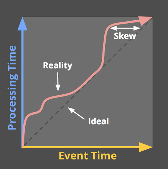
The black dashed line with a slope of one represents the ideal, where processing time and event time are exactly equal; the red line represents reality. In this example, the system lags a bit at the beginning of processing time, veers closer toward the ideal in the middle, then lags again a bit toward the end. The horizontal distance between the ideal and the red line is the skew between processing time and event time. That skew is essentially the latency introduced by the processing pipeline.
Since the mapping between event time and processing time is not static, this means you cannot analyze your data solely within the context of when they are observed in your pipeline if you care about their event times (i.e., when the events actually occurred). Unfortunately, this is the way most existing systems designed for unbounded data operate. To cope with the infinite nature of unbounded data sets, these systems typically provide some notion of windowing the incoming data. We’ll discuss windowing in great depth below, but it essentially means chopping up a data set into finite pieces along temporal boundaries.
If you care about correctness and are interested in analyzing your data in the context of their event times, you cannot define those temporal boundaries using processing time (i.e., processing time windowing), as most existing systems do; with no consistent correlation between processing time and event time, some of your event time data are going to end up in the wrong processing time windows (due to the inherent lag in distributed systems, the online/offline nature of many types of input sources, etc.), throwing correctness out the window, as it were. We’ll look at this problem in more detail in a number of examples below as well as in the next post.
Unfortunately, the picture isn’t exactly rosy when windowing by event time, either. In the context of unbounded data, disorder and variable skew induce a completeness problem for event time windows: lacking a predictable mapping between processing time and event time, how can you determine when you’ve observed all the data for a given event time X? For many real-world data sources, you simply can’t. The vast majority of data processing systems in use today rely on some notion of completeness, which puts them at a severe disadvantage when applied to unbounded data sets.
I propose that instead of attempting to groom unbounded data into finite batches of information that eventually become complete, we should be designing tools that allow us to live in the world of uncertainty imposed by these complex data sets. New data will arrive, old data may be retracted or updated, and any system we build should be able to cope with these facts on its own, with notions of completeness being a convenient optimization rather than a semantic necessity.
Before diving into how we’ve tried to build such a system with the Dataflow Model used in Cloud Dataflow, let’s finish up one more useful piece of background: common data processing patterns.
Data processing patterns
At this point in time, we have enough background established that we can start looking at the core types of usage patterns common across bounded and unbounded data processing today. We’ll look at both types of processing, and where relevant, within the context of the two main types of engines we care about (batch and streaming, where in this context, I’m essentially lumping micro-batch in with streaming since the differences between the two aren’t terribly important at this level).
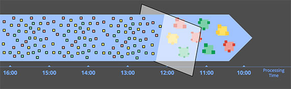
Bounded data
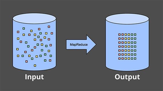
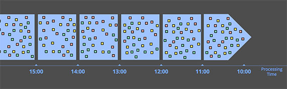
Processing bounded data is quite straightforward, and likely familiar to everyone. In the diagram below, we start out on the left with a data set full of entropy. We run it through some data processing engine (typically batch, though a well-designed streaming engine would work just as well), such as MapReduce, and on the right end up with a new structured data set with greater inherent value:
Though there are, of course, infinite variations on what you can actually calculate as part of this scheme, the overall model is quite simple. Much more interesting is the task of processing an unbounded data set. Let’s now look at the various ways unbounded data are typically processed, starting with the approaches used with traditional batch engines, and then ending up with the approaches one can take with a system designed for unbounded data, such as most streaming or micro-batch engines.
Unbounded data — batch
Batch engines, though not explicitly designed with unbounded data in mind, have been used to process unbounded data sets since batch systems were first conceived. As one might expect, such approaches revolve around slicing up the unbounded data into a collection of bounded data sets appropriate for batch processing.
Fixed windows
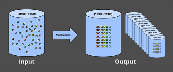
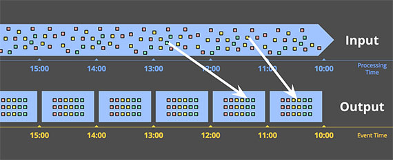
The most common way to process an unbounded data set using repeated runs of a batch engine is by windowing the input data into fixed-sized windows, then processing each of those windows as a separate, bounded data source. Particularly for input sources like logs, where events can be written into directory and file hierarchies whose names encode the window they correspond to, this sort of thing appears quite straightforward at first blush since you’ve essentially performed the time-based shuffle to get data into the appropriate event time windows ahead of time.
In reality, however, most systems still have a completeness problem to deal with: what if some of your events are delayed en route to the logs due to a network partition? What if your events are collected globally and must be transferred to a common location before processing? What if your events come from mobile devices? This means some sort of mitigation may be necessary (e.g., delaying processing until you’re sure all events have been collected, or re-processing the entire batch for a given window whenever data arrive late).
Sessions
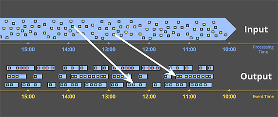
This approach breaks down even more when you try to use a batch engine to process unbounded data into more sophisticated windowing strategies, like sessions. Sessions are typically defined as periods of activity (e.g., for a specific user) terminated by a gap of inactivity. When calculating sessions using a typical batch engine, you often end up with sessions that are split across batches, as indicated by the red marks in the diagram below. The number of splits can be reduced by increasing batch sizes, but at the cost of increased latency. Another option is to add additional logic to stitch up sessions from previous runs, but at the cost of further complexity.
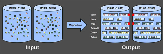
Either way, using a classic batch engine to calculate sessions is less than ideal. A nicer way would be to build up sessions in a streaming manner, which we’ll look at later on.
Unbounded data — streaming
Contrary to the ad hoc nature of most batch-based unbounded data processing approaches, streaming systems are built for unbounded data. As I noted earlier, for many real-world, distributed input sources, you not only find yourself dealing with unbounded data, but also data that are:
- Highly unordered with respect to event times, meaning you need some sort of time-based shuffle in your pipeline if you want to analyze the data in the context in which they occurred.
- Of varying event time skew, meaning you can’t just assume you’ll always see most of the data for a given event time X within some constant epsilon of time Y.
There are a handful of approaches one can take when dealing with data that have these characteristics. I generally categorize these approaches into four groups:
- Time-agnostic
- Approximation
- Windowing by processing time
- Windowing by event time
We’ll now spend a little bit of time looking at each of these approaches.
Time-agnostic
Time-agnostic processing is used in cases where time is essentially irrelevant — i.e., all relevant logic is data driven. Since everything about such use cases is dictated by the arrival of more data, there’s really nothing special a streaming engine has to support other than basic data delivery. As a result, essentially all streaming systems in existence support time-agnostic use cases out of the box (modulo system-to-system variances in consistency guarantees, of course, for those of you that care about correctness). Batch systems are also well suited for time-agnostic processing of unbounded data sources, by simply chopping the unbounded source into an arbitrary sequence of bounded data sets and processing those data sets independently. We’ll look at a couple of concrete examples in this section, but given the straightforwardness of handling time-agnostic processing, won’t spend much more time on it beyond that.
Filtering
A very basic form of time-agnostic processing is filtering. Imagine you’re processing Web traffic logs, and you want to filter out all traffic that didn’t originate from a specific domain. You would look at each record as it arrived, see if it belonged to the domain of interest, and drop it if not. Since this sort of thing depends only on a single element at any time, the fact that the data source is unbounded, unordered, and of varying event time skew is irrelevant.
Inner-joins
Another time-agnostic example is an inner-join (or hash-join). When joining two unbounded data sources, if you only care about the results of a join when an element from both sources arrive, there’s no temporal element to the logic. Upon seeing a value from one source, you can simply buffer it up in persistent state; you only need to emit the joined record once the second value from the other source arrives. (In truth, you’d likely want some sort of garbage collection policy for unemitted partial joins, which would likely be time based. But for a use case with little or no uncompleted joins, such a thing might not be an issue.)
Switching semantics to some sort of outer join introduces the data completeness problem we’ve talked about: once you’ve seen one side of the join, how do you know whether the other side is ever going to arrive or not? Truth be told, you don’t, so you have to introduce some notion of a timeout, which introduces an element of time. That element of time is essentially a form of windowing, which we’ll look at more closely in a moment.
Approximation algorithms
The second major category of approaches is approximation algorithms, such as approximate Top-N, streaming K-means, etc. They take an unbounded source of input and provide output data that, if you squint at them, look more or less like what you were hoping to get. The upside of approximation algorithms is that, by design, they are low overhead and designed for unbounded data. The downsides are that a limited set of them exist, the algorithms themselves are often complicated (which makes it difficult to conjure up new ones), and their approximate nature limits their utility.
It’s worth noting: these algorithms typically do have some element of time in their design (e.g., some sort of built-in decay). And since they process elements as they arrive, that element of time is usually processing-time based. This is particularly important for algorithms that provide some sort of provable error bounds on their approximations. If those error bounds are predicated on data arriving in order, they mean essentially nothing when you feed the algorithm unordered data with varying event-time skew. Something to keep in mind.
Approximation algorithms themselves are a fascinating subject, but as they are essentially another example of time-agnostic processing (modulo the temporal features of the algorithms themselves), they’re quite straightforward to use, and thus not worth further attention given our current focus.
Windowing
The remaining two approaches for unbounded data processing are both variations of windowing. Before diving into the differences between them, I should make it clear exactly what I mean by windowing since I’ve only touched on it briefly. Windowing is simply the notion of taking a data source (either unbounded or bounded), and chopping it up along temporal boundaries into finite chunks for processing. The following diagram shows three different windowing patterns:
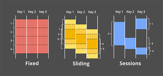
- Fixed windows: Fixed windows slice up time into segments with a fixed-size temporal length. Typically (as in Figure 8), the segments for fixed windows are applied uniformly across the entire data set, which is an example of aligned windows. In some cases, it’s desirable to phase-shift the windows for different subsets of the data (e.g., per key) to spread window completion load more evenly over time, which instead is an example of unaligned windows since they vary across the data.
- Sliding windows: A generalization of fixed windows, sliding windows are defined by a fixed length and a fixed period. If the period is less than the length, then the windows overlap. If the period equals the length, you have fixed windows. And if the period is greater than the length, you have a weird sort of sampling window that only looks at subsets of the data over time. As with fixed windows, sliding windows are typically aligned, though may be unaligned as a performance optimization in certain use cases. Note that the sliding windows in the Figure 8 are drawn as they are to give a sense of sliding motion; in reality, all five windows would apply across the entire data set.
- Sessions: An example of dynamic windows, sessions are composed of sequences of events terminated by a gap of inactivity greater than some timeout. Sessions are commonly used for analyzing user behavior over time, by grouping together a series of temporally-related events (e.g., a sequence of videos viewed in one sitting). Sessions are interesting because their lengths cannot be defined a priori; they are dependent upon the actual data involved. They’re also the canonical example of unaligned windows since sessions are practically never identical across different subsets of data (e.g., different users).
The two domains of time discussed — processing time and event time — are essentially the two we care about[2]. Windowing makes sense in both domains, so we’ll look at each in detail and see how they differ. Since processing time windowing is vastly more common in existing systems, I’ll start there.
Windowing by processing time
When windowing by processing time, the system essentially buffers up incoming data into windows until some amount of processing time has passed. For example, in the case of five-minute fixed windows, the system would buffer up data for five minutes of processing time, after which it would treat all the data it had observed in those five minutes as a window and send them downstream for processing.
There are a few nice properties of processing time windowing:
- It’s simple. The implementation is extremely straightforward since you never worry about shuffling data within time. You just buffer things up as they arrive and send them downstream when the window closes.
- Judging window completeness is straightforward. Since the system has perfect knowledge of whether all inputs for a window have been seen or not, it can make perfect decisions about whether a given window is complete or not. This means there is no need to be able to deal with “late” data in any way when windowing by processing time.
- If you’re wanting to infer information about the source as it is observed, processing time windowing is exactly what you want. Many monitoring scenarios fall into this category. Imagine tracking the number of requests per second sent to a global-scale Web service. Calculating a rate of these requests for the purpose of detecting outages is a perfect use of processing time windowing.
Good points aside, there is one very big downside to processing time windowing: if the data in question have event times associated with them, those data must arrive in event time order if the processing time windows are to reflect the reality of when those events actually happened. Unfortunately, event-time ordered data are uncommon in many real-world, distributed input sources.
As a simple example, imagine any mobile app that gathers usage statistics for later processing. In cases where a given mobile device goes offline for any amount of time (brief loss of connectivity, airplane mode while flying across the country, etc.), the data recorded during that period won’t be uploaded until the device comes online again. That means data might arrive with an event time skew of minutes, hours, days, weeks, or more. It’s essentially impossible to draw any sort of useful inferences from such a data set when windowed by processing time.
As another example, many distributed input sources may seem to provide event-time ordered (or very nearly so) data when the overall system is healthy. Unfortunately, the fact that event-time skew is low for the input source when healthy does not mean it will always stay that way. Consider a global service that processes data collected on multiple continents. If network issues across a bandwidth-constrained transcontinental line (which, sadly, are surprisingly common) further decrease bandwidth and/or increase latency, suddenly a portion of your input data may start arriving with much greater skew than before. If you are windowing that data by processing time, your windows are no longer representative of the data that actually occurred within them; instead, they represent the windows of time as the events arrived at the processing pipeline, which is some arbitrary mix of old and current data.
What we really want in both of those cases is to window data by their event times in a way that is robust to the order of arrival of events. What we really want is event time windowing.
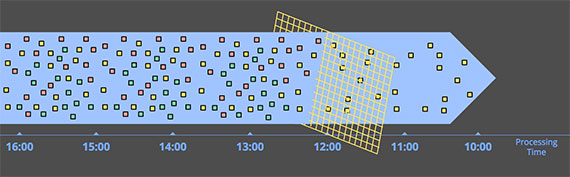
Windowing by event time
Event time windowing is what you use when you need to observe a data source in finite chunks that reflect the times at which those events actually happened. It’s the gold standard of windowing. Sadly, most data processing systems in use today lack native support for it (though any system with a decent consistency model, like Hadoop or Spark Streaming, could act as a reasonable substrate for building such a windowing system).
This diagram shows an example of windowing an unbounded source into one-hour fixed windows:
The solid white lines in the diagram call out two particular data of interest. Those two data both arrived in processing time windows that did not match the event time windows to which they belonged. As such, if these data had been windowed into processing time windows for a use case that cared about event times, the calculated results would have been incorrect. As one would expect, event time correctness is one nice thing about using event time windows.
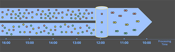
Another nice thing about event time windowing over an unbounded data source is that you can create dynamically sized windows, such as sessions, without the arbitrary splits observed when generating sessions over fixed windows (as we saw previously in the sessions example from the “Unbounded data — batch” section):
Of course, powerful semantics rarely come for free, and event time windows are no exception. Event time windows have two notable drawbacks due to the fact that windows must often live longer (in processing time) than the actual length of the window itself:
- Buffering: Due to extended window lifetimes, more buffering of data is required. Thankfully, persistent storage is generally the cheapest of the resource types most data processing systems depend on (the others being primarily CPU, network bandwidth, and RAM). As such, this problem is typically much less of a concern than one might think when using any well-designed data-processing system with strongly consistent persistent state and a decent in-memory caching layer. Also, many useful aggregations do not require the entire input set to be buffered (e.g., sum, or average), but instead can be performed incrementally, with a much smaller, intermediate aggregate stored in persistent state.
- Completeness: Given that we often have no good way of knowing when we’ve seen all the data for a given window, how do we know when the results for the window are ready to materialize? In truth, we simply don’t. For many types of inputs, the system can give a reasonably accurate heuristic estimate of window completion via something like MillWheel’s watermarks (which I’ll talk about more in Part 2). But in cases where absolute correctness is paramount (again, think billing), the only real option is to provide a way for the pipeline builder to express when they want results for windows to be materialized, and how those results should be refined over time. Dealing with window completeness (or lack, thereof), is a fascinating topic, but one perhaps best explored in the context of concrete examples, which we’ll look at next time.
Conclusion
Whew! That was a lot of information. To those of you that have made it this far: you are to be commended! At this point we are roughly halfway through the material I want to cover, so it’s probably reasonable to step back, recap what I’ve covered so far, and let things settle a bit before diving into Part 2. The upside of all this is that Part 1 is the boring post; Part 2 is where the fun really begins.
Recap
To summarize, in this post I’ve:
- Clarified terminology, specifically narrowing the definition of “streaming” to apply to execution engines only, while using more descriptive terms like unbounded data and approximate/speculative results for distinct concepts often categorized under the “streaming” umbrella.
- Assessed the relative capabilities of well-designed batch and streaming systems, positing that streaming is in fact a strict superset of batch, and that notions like the Lambda Architecture, which are predicated on streaming being inferior to batch, are destined for retirement as streaming systems mature.
- Proposed two high-level concepts necessary for streaming systems to both catch up to and ultimately surpass batch, those being correctness and tools for reasoning about time, respectively.
- Established the important differences between event time and processing time, characterized the difficulties those differences impose when analyzing data in the context of when they occurred, and proposed a shift in approach away from notions of completeness and toward simply adapting to changes in data over time.
- Looked at the major data processing approaches in common use today for bounded and unbounded data, via both batch and streaming engines, roughly categorizing the unbounded approaches into: time-agnostic, approximation, windowing by processing time, and windowing by event time.
Next time
This post provides the context necessary for the concrete examples I’ll be exploring in Part 2. That post will consist of roughly the following:
- A conceptual look at how we’ve broken up the notion of data processing in the Dataflow Model across four related axes: what, where, when, and how.
- A detailed look at processing a simple, concrete example data set across multiple scenarios, highlighting the plurality of use cases enabled by the Dataflow Model, and the concrete APIs involved. These examples will help drive home the notions of event time and processing time introduced in this post, while additionally exploring new concepts, such as watermarks.
- A comparison of existing data-processing systems across the important characteristics covered in both posts, to better enable educated choice amongst them, and to encourage improvement in areas that are lacking, with my ultimate goal being the betterment of data processing systems in general, and streaming systems in particular, across the entire big data community.
Should be a good time. See you then!