Using TensorFlow to generate images with PixelRNNs
Generate new images and fix old ones using neural networks.
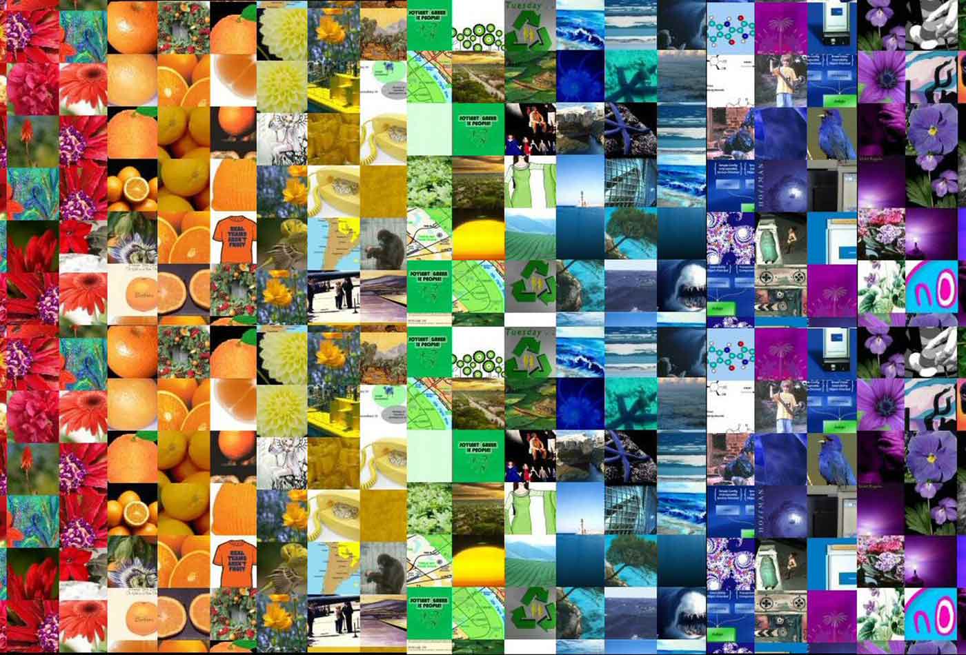 Montage (source: Mary-Lynn on Flickr)
Pixel Recurrent Neural Networks (PixelRNNs) combine a number of techniques to generate natural-looking images using neural networks. PixelRNNs model the distribution of image data sets using several new techniques, including a novel spatial LSTM cell, and sequentially infer the pixels in an image to (a) generate novel images or (b) predict unseen pixels to complete an occluded image.
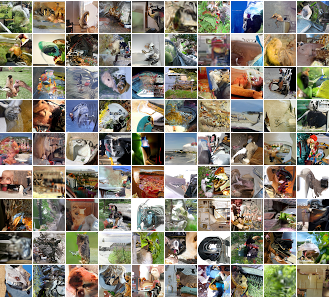
The images in Figure 1 were produced by a PixelRNN model trained on the 32×32 ImageNet data set. In this article, we will create a PixelRNN to generate images from the MNIST data set. You can follow along in the article, or check out our Jupyter Notebook.

Learn faster. Dig deeper. See farther.
Before we get started, you’ll need to install TensorFlow (TF) for Python. Check the instructions, but for most people, it should be as easy as running:
pip install tensorflow
If you haven’t had a chance to work with TF before, we recommend the O’Reilly article, Hello, TensorFlow! Building and training your first TensorFlow model.
Generative image models and prior work
We mentioned earlier that the PixelRNN is a generative model. A generative model attempts to model the joint probability distribution of the data we feed in. In the context of PixelRNN, this basically means we want to model all of the possible realistic images as compactly as possible. Doing so would allow us to generate novel images from this distribution. Modeling the distribution of natural images is a landmark problem in machine learning. Several other neural network architectures have attempted to achieve this task, including Generative Adversarial Networks (A. Redford, et. al.), Variational Autoencoders (Y. Pu, et. al.), and spatial LSTM networks (L. Theis, et. al).
PixelRNN generative model
To model the distribution of images, PixelRNNs make the following assumption about pixel intensities: the intensity value of a pixel is dependent on all pixels traversed before it. The image is traversed left-to-right and top-to-bottom along the image.
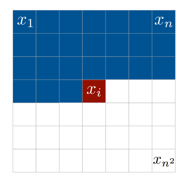
In an \(nxn\) image, we have that the intensity for pixel \(x_i\) is conditioned on all preceding pixels: \(x_j, 0 \lt j \gt i\), or in other terms:
$$x_i \sim p(x_i | x_1, x_2, \cdots, x_{i-1})$$
We calculate the joint probability of an image x by multiplying all conditional probabilities of the image togther, as so:
$$p(x) = \prod_{i=1}^{n^2} p(x_i | x_1, \cdots, x_{i-1})$$
We learn these conditional probabilities through a series of special convolutions that capture this context around a given pixel.
Diagonal BiLSTMs and convolutions
LSTM cells used by the main variant of PixelRNNs capture this conditional dependency across dozens or hundreds of pixels. In the paper by Google DeepMind, the authors implement a novel spatial bi-directional LSTM cell, the Diagonal BiLSTM, to capture the desired spatial context of a pixel.
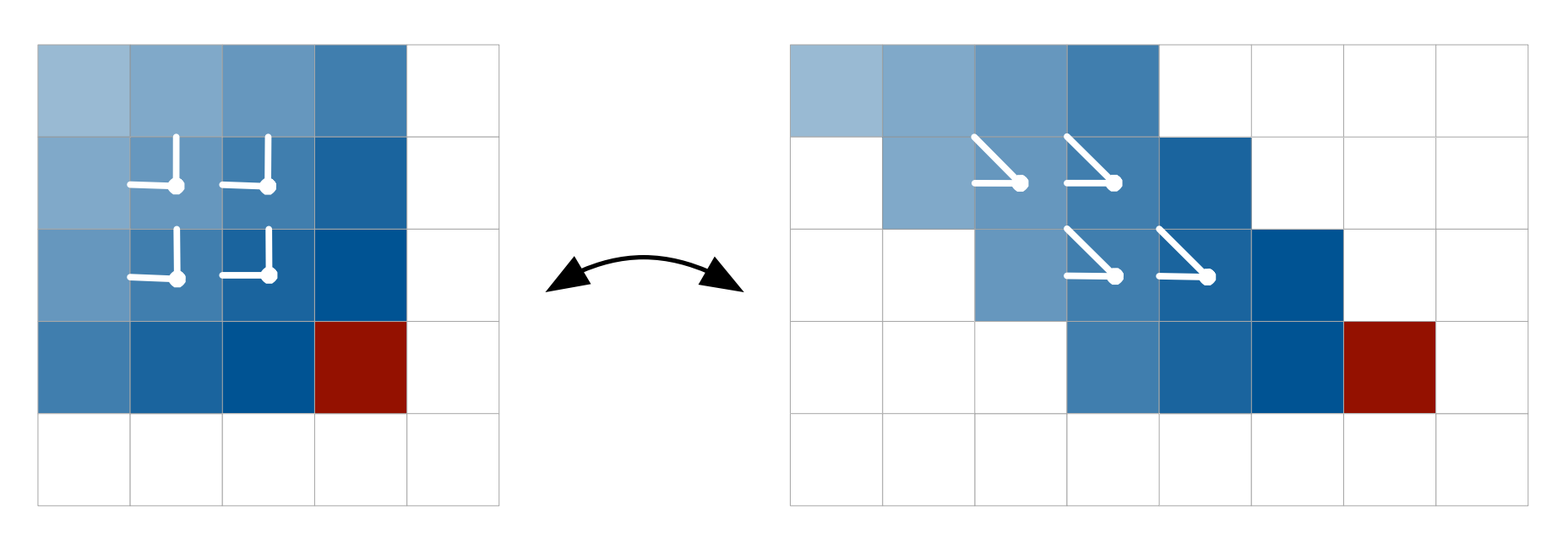
To aid in capturing context before the first layer of the network, we mask the input image so that for a given pixel \(x_i\) we are predicting, we set the values of all pixels yet to be traversed, \(x_j, j \ge i,\) to 0, to prevent them from contributing to the overall prediction. In subsequent LSTM layers, we perform a similar mask, but no longer set \(x_i\) to 0 in the mask. We then skew the image, so that each row is offset by one from the row above it, as shown above. We can then perform a series of k x 1 convolutions on the skewed image using the Diagonal BiLSTM cells.
This enables us to efficiently capture the preceding pixels in the image to predict the upcoming one. LSTM cells also capture a potentially unbounded dependency range between pixels in their receptive field. However, this comes at a high computational cost, as the LSTM requires “unrolling” a layer many steps into the future. This begs the question: can we do something more efficient?
A faster method—computing many features at once
A faster alternative architecture involves replacing the LSTM cell with a series of convolutions to capture a large, but bounded receptive field. This allows us to compute the features contained within the receptive field at once, and avoids the computational cost of sequentially computing each cell’s hidden state.
We can implement the convolution operation like so, performing the masks as needed (access the notebook for this article here):
def conv2d(
    inputs,
    num_outputs,
    kernel_shape, # [kernel_height, kernel_width]
    mask_type, # None, "A" or "B",
    strides=[1, 1], # [column_wise_stride, row_wise_stride]
    padding="SAME",
    activation_fn=None,
    weights_initializer=tf.contrib.layers.xavier_initializer(),
    weights_regularizer=None,
    biases_initializer=tf.zeros_initializer,
    biases_regularizer=None,
    scope="conv2d"):
  with tf.variable_scope(scope):
    batch_size, height, width, channel = inputs.get_shape().as_list()
    kernel_h, kernel_w = kernel_shape
    stride_h, stride_w = strides

    center_h = kernel_h // 2
    center_w = kernel_w // 2
Here, we use the Xavier weights initialization scheme (X. Glorot and Y. Bengio) to create the convolution kernel.
    weights_shape = [kernel_h, kernel_w, channel, num_outputs]
    weights = tf.get_variable("weights", weights_shape,
      tf.float32, weights_initializer, weights_regularizer)
Next, we apply the mask to the image to restrict the focus of the kernel to the current context.
    if mask_type is not None:
      mask = np.ones(
        (kernel_h, kernel_w, channel, num_outputs), dtype=np.float32)

      mask[center_h, center_w+1: ,: ,:] = 0.
      mask[center_h+1:, :, :, :] = 0.

      if mask_type == 'a':
        mask[center_h,center_w,:,:] = 0.

      weights *= tf.constant(mask, dtype=tf.float32)
      tf.add_to_collection('conv2d_weights_%s' % mask_type, weights)
Finally, we apply the convolution to the image and apply an optional activation function like ReLU.
    outputs = tf.nn.conv2d(inputs,
        weights, [1, stride_h, stride_w, 1], padding=padding, name='outputs')
    tf.add_to_collection('conv2d_outputs', outputs)

    if biases_initializer != None:
      biases = tf.get_variable("biases", [num_outputs,],
          tf.float32, biases_initializer, biases_regularizer)
      outputs = tf.nn.bias_add(outputs, biases, name='outputs_plus_b')

    if activation_fn:
      outputs = activation_fn(outputs, name='outputs_with_fn')
    return outputs
Generating images with MNIST
For this article, we will train our PixelRNN on the MNIST data set. Then, we’ll draw from the
PixelRNNs model to generate handwritten digits that don’t appear in our data set. You can download the data set here—however, if you use the load_data() function from utils.py, you won’t have to worry about this. We’ll also demonstrate the PixelRNNs ability to complete a partially occluded image by predicting the rest of the pixels.
Features of the network
In place of Diagonal BiLSTM layers, we use the convolutions described earlier.
In addition to the convolutional layers, PixelRNNs also makes use of residual connections (He, et. al.). Residual connections effectively copy the output from early layers in the network and concatenate this with the output of a deeper layer. This helps preserve information learned earlier in the model. For the convolutional layers in our model, these residual connections look something like this:
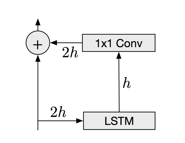
The residual connections allow our model to increase in depth and still gain accuracy, while simultaneously making the model easier to optimize.
The final layer applies a sigmoid activation function on the input. This layer outputs a value between 0 and 1 that is the resulting normalized pixel intensity.
With this in mind, the final architecture looks like this:
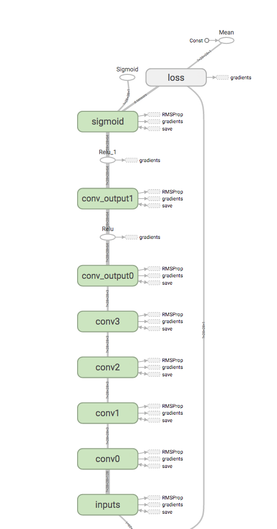
Using this architecture and the convolution operations described above, we can construct the network.
def pixelRNN(height, width, channel, params):
    """
    Args
    height, width, channel - the dimensions of the input
    params the hyperparameters of the network
    """
    input_shape = [None, height, width, channel]
    inputs = tf.placeholder(tf.float32, input_shape)
Here we apply a 7×7 convolution to the image while applying the initial A mask that removes the self-connection to the pixel being predicted.
    # input of main recurrent layers
    scope = "conv_inputs"
    conv_inputs = conv2d(inputs, params.hidden_dims, [7, 7], "A", scope=scope)
Next, we construct a series of 1×1 convolutions to apply to the image.
    # main recurrent layers
    last_hid = conv_inputs
    for idx in xrange(params.recurrent_length):
        scope = 'CONV%d' % idx
        last_hid = conv2d(last_hid, 3, [1, 1], "B", scope=scope)
        print("Building %s" % scope)
Then, we construct another series of 1×1 convolutions using ReLU activation.
    # output recurrent layers
    for idx in xrange(params.out_recurrent_length):
        scope = 'CONV_OUT%d' % idx
        last_hid = tf.nn.relu(conv2d(last_hid, params.out_hidden_dims, [1, 1], "B", scope=scope))
        print("Building %s" % scope)
Finally, we apply one final convolution layer with a sigmoid activation to produce a series of pixel predictions for the image.
    conv2d_out_logits = conv2d(last_hid, 1, [1, 1], "B", scope='conv2d_out_logits')
    output = tf.nn.sigmoid(conv2d_out_logits)
    return inputs, output, conv2d_out_logits
inputs, output, conv2d_out_logits = pixelRNN(height, width, channel, p)
Training procedure
To train the network, we supply mini-batches of binarized images and predict each pixel in parallel using our network. We minimize the cross entropy between our predictions and the binary pixel values of the images. We optimize this objective using an RMSProp optimizer with a learning rate of 0.001, selected using grid search. The Google DeepMind paper lists RMSProp optimization as the empirically most effective optimizer through all experiments. In practice, we find that clipping the gradients helps stabilize learning. We use a batch size of 100 and 16 hidden units for each convolution.
Let’s optimize the network we constructed above using this procedure:
loss = tf.reduce_mean(tf.nn.sigmoid_cross_entropy_with_logits(conv2d_out_logits, inputs, name='loss'))

optimizer = tf.train.RMSPropOptimizer(p.learning_rate)
grads_and_vars = optimizer.compute_gradients(loss)

new_grads_and_vars = \
    [(tf.clip_by_value(gv[0], -p.grad_clip, p.grad_clip), gv[1]) for gv in grads_and_vars]
optim = optimizer.apply_gradients(new_grads_and_vars)
Generation and occlusion completion
After training the network, we can use the resulting model to generate sample images using the generative model we’ve described. We can also infer the remaining pixel values in a partially occluded image to complete it. The code to do so is fairly simple:
def predict(sess, images, inputs, output):
    return sess.run(output, {inputs: images})

def generate(sess, height, width, inputs, output):
    samples = np.zeros((100, height, width, 1), dtype='float32')

    for i in range(height):
        for j in range(width):
            next_sample = binarize(predict(sess, samples, inputs, output))
            samples[:, i, j] = next_sample[:, i, j]

    return samples

def generate_occlusions(sess, height, width, inputs, output):
    samples = occlude(images, height, width)
    starting_position = [0,height//2]
    for i in range(starting_position[1], height):
        for j in range(starting_position[0], width):
            next_sample = binarize(predict(sess, samples, inputs, output))
            samples[:, i, j] = next_sample[:, i, j]
    return samples
We can complete occluded images by using the same generative procedure, only modifying the starting point.
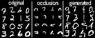
As you can see, the algorithm can successfully finish an occluded image. Clearly, there are some discrepancies in the generated numbers and the original numbers. For example, the 7 in the top left becomes a 9 in the generated image. However, these mistakes are not unreasonable—the curve that remains after the occlusion could arbitrarily belong to several different handwritten digits.
Next steps
The PixelRNN framework provides a useful architecture for generating modeling. Although we implement a single color channel version for MNIST, Google DeepMind’s original paper discusses a slightly more sophisticated architecture that can deal with multi-channel color images. This system can model more complex data sets like CIFAR10 and ImageNet. The TensorFlow Magenta team has an excellent review that explains the mathematics behind this algorithm at a higher level than the paper.
What we’ve shown here is a benchmark with a very simple data set using a relatively fast model that can learn the distribution of MNIST images. Next steps might include extending this model to work with images composed of multiple color channels, like CIFAR10.
Another option is to implement the original Diagonal BiLSTM cell in place of the faster convolutions. This implementation is much more computationally expensive—even on a state-of-the-art GPU. We found in practice that the convolution-based architecture ran approximately 20x faster than the Diagonal BiLSTM one.
Further work on the convolution-based architecture, PixelCNN, can be found in the paper Conditional Image Generation with PixelCNN Decoders. OpenAI recently went a step further and open sourced a repo that implements a computationally faster version of the above paper using several significant architecture improvements.
Don’t forget to check out our notebook and repo to play around with this code yourself! As a note, if you don’t own a GPU, you can rent one from AWS for cheap. Phillip wrote a guide on how to start an AWS EC2 instance for deep learning—including how to set up a Jupyter Notebook server.
This post is a collaboration between O’Reilly and TensorFlow. See our statement of editorial independence.