Hello, TensorFlow!

The TensorFlow project is bigger than you might realize. The fact that it’s a library for deep learning, and its connection to Google, has helped TensorFlow attract a lot of attention. But beyond the hype, there are unique elements to the project that are worthy of closer inspection:

• The core library is suited to a broad family of machine learning techniques, not “just” deep learning.
• Linear algebra and other internals are prominently exposed.
• In addition to the core machine learning functionality, TensorFlow also includes its own logging system, its own interactive log visualizer, and even its own heavily engineered serving architecture.
• The execution model for TensorFlow differs from Python’s scikit-learn, or most tools in R.

Cool stuff, but—especially for someone hoping to explore machine learning for the first time—TensorFlow can be a lot to take in.

How does TensorFlow work? Let’s break it down so we can see and understand every moving part. We’ll explore the data flow graph that defines the computations your data will undergo, how to train models with gradient descent using TensorFlow, and how TensorBoard can visualize your TensorFlow work. The examples here won’t solve industrial machine learning problems, but they’ll help you understand the components underlying everything built with TensorFlow, including whatever you build next!

Names and execution in Python and TensorFlow

The way TensorFlow manages computation is not totally different from the way Python usually does. With both, it’s important to remember, to paraphrase Hadley Wickham, that an object has no name (see Figure 1). In order to see the similarities (and differences) between how Python and TensorFlow work, let’s look at how they refer to objects and handle evaluation.

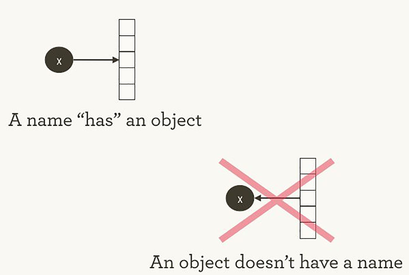
The variable names in Python code aren’t what they represent; they’re just pointing at objects. So, when you say in Python that foo = [] and bar = foo, it isn’t just that foo equals bar; foo is bar, in the sense that they both point at the same list object.

>>> foo = []
>>> bar = foo
>>> foo == bar
## True
>>> foo is bar
## True

You can also see that id(foo) and id(bar) are the same. This identity, especially with mutable data structures like lists, can lead to surprising bugs when it’s misunderstood.

Internally, Python manages all your objects and keeps track of your variable names and which objects they refer to. The TensorFlow graph represents another layer of this kind of management; as we’ll see, Python names will refer to objects that connect to more granular and managed TensorFlow graph operations.

When you enter a Python expression, for example at an interactive interpreter or Read Evaluate Print Loop (REPL), whatever is read is almost always evaluated right away. Python is eager to do what you tell it. So, if I tell Python to foo.append(bar), it appends right away, even if I never use foo again.

A lazier alternative would be to just remember that I said foo.append(bar), and if I ever evaluate foo at some point in the future, Python could do the append then. This would be closer to how TensorFlow behaves, where defining relationships is entirely separate from evaluating what the results are.

TensorFlow separates the definition of computations from their execution even further by having them happen in separate places: a graph defines the operations, but the operations only happen within a session. Graphs and sessions are created independently. A graph is like a blueprint, and a session is like a construction site.

Back to our plain Python example, recall that foo and bar refer to the same list. By appending bar into foo, we’ve put a list inside itself. You could think of this structure as a graph with one node, pointing to itself. Nesting lists is one way to represent a graph structure like a TensorFlow computation graph.

>>> foo.append(bar)
>>> foo
## [[...]]

Real TensorFlow graphs will be more interesting than this!

The simplest TensorFlow graph

To start getting our hands dirty, let’s create the simplest TensorFlow graph we can, from the ground up. TensorFlow is admirably easier to install than some other frameworks. The examples here work with either Python 2.7 or 3.3+, and the TensorFlow version used is 0.8.

>>> import tensorflow as tf

At this point TensorFlow has already started managing a lot of state for us. There’s already an implicit default graph, for example. Internally, the default graph lives in the _default_graph_stack, but we don’t have access to that directly. We use tf.get_default_graph().

>>> graph = tf.get_default_graph()

The nodes of the TensorFlow graph are called “operations,” or “ops.” We can see what operations are in the graph with graph.get_operations().

>>> graph.get_operations()
## []

Currently, there isn’t anything in the graph. We’ll need to put everything we want TensorFlow to compute into that graph. Let’s start with a simple constant input value of one.

>>> input_value = tf.constant(1.0)

That constant now lives as a node, an operation, in the graph. The Python variable name input_value refers indirectly to that operation, but we can also find the operation in the default graph.

>>> operations = graph.get_operations()
>>> operations
## [<tensorflow.python.framework.ops.Operation at 0x1185005d0>]
>>> operations[0].node_def
## name: "Const"
## op: "Const"
## attr {
##   key: "dtype"
##   value {
##     type: DT_FLOAT
##   }
## }
## attr {
##   key: "value"
##   value {
##     tensor {
##       dtype: DT_FLOAT
##       tensor_shape {
##       }
##       float_val: 1.0
##     }
##   }
## }

TensorFlow uses protocol buffers internally. (Protocol buffers are sort of like a Google-strength JSON.) Printing the node_def for the constant operation above shows what’s in TensorFlow’s protocol buffer representation for the number one.

People new to TensorFlow sometimes wonder why there’s all this fuss about making “TensorFlow versions” of things. Why can’t we just use a normal Python variable without also defining a TensorFlow object? One of the TensorFlow tutorials has an explanation:

To do efficient numerical computing in Python, we typically use libraries like NumPy that do expensive operations such as matrix multiplication outside Python, using highly efficient code implemented in another language. Unfortunately, there can still be a lot of overhead from switching back to Python every operation. This overhead is especially bad if you want to run computations on GPUs or in a distributed manner, where there can be a high cost to transferring data.

TensorFlow also does its heavy lifting outside Python, but it takes things a step further to avoid this overhead. Instead of running a single expensive operation independently from Python, TensorFlow lets us describe a graph of interacting operations that run entirely outside Python. This approach is similar to that used in Theano or Torch.

TensorFlow can do a lot of great things, but it can only work with what’s been explicitly given to it. This is true even for a single constant.

If we inspect our input_value, we see it is a constant 32-bit float tensor of no dimension: just one number.

>>> input_value
## <tf.Tensor 'Const:0' shape=() dtype=float32>

Note that this doesn’t tell us what that number is. To evaluate input_value and get a numerical value out, we need to create a “session” where graph operations can be evaluated and then explicitly ask to evaluate or “run” input_value. (The session picks up the default graph by default.)

>>> sess = tf.Session()
>>> sess.run(input_value)
## 1.0

It may feel a little strange to “run” a constant. But it isn’t so different from evaluating an expression as usual in Python; it’s just that TensorFlow is managing its own space of things—the computational graph—and it has its own method of evaluation.

The simplest TensorFlow neuron

Now that we have a session with a simple graph, let’s build a neuron with just one parameter, or weight. Often, even simple neurons also have a bias term and a non-identity activation function, but we’ll leave these out.

The neuron’s weight isn’t going to be constant; we expect it to change in order to learn based on the “true” input and output we use for training. The weight will be a TensorFlow variable. We’ll give that variable a starting value of 0.8.

>>> weight = tf.Variable(0.8)

You might expect that adding a variable would add one operation to the graph, but in fact that one line adds four operations. We can check all the operation names:

>>> for op in graph.get_operations(): print(op.name)
## Const
## Variable/initial_value
## Variable
## Variable/Assign
## Variable/read

We won’t want to follow every operation individually for long, but it will be nice to see at least one that feels like a real computation.

>>> output_value = weight * input_value

Now there are six operations in the graph, and the last one is that multiplication.

>>> op = graph.get_operations()[-1]
>>> op.name
## 'mul'
>>> for op_input in op.inputs: print(op_input)
## Tensor("Variable/read:0", shape=(), dtype=float32)
## Tensor("Const:0", shape=(), dtype=float32)

This shows how the multiplication operation tracks where its inputs come from: they come from other operations in the graph. To understand a whole graph, following references this way quickly becomes tedious for humans. TensorBoard graph visualization is designed to help.

How do we find out what the product is? We have to “run” the output_value operation. But that operation depends on a variable: weight. We told TensorFlow that the initial value of weight should be 0.8, but the value hasn’t yet been set in the current session. The tf.initialize_all_variables() function generates an operation which will initialize all our variables (in this case just one) and then we can run that operation.

>>> init = tf.initialize_all_variables()
>>> sess.run(init)

The result of tf.initialize_all_variables() will include initializers for all the variables currently in the graph, so if you add more variables you’ll want to use tf.initialize_all_variables() again; a stale init wouldn’t include the new variables.

Now we’re ready to run the output_value operation.

>>> sess.run(output_value)
## 0.80000001

Recall that’s 0.8 * 1.0 with 32-bit floats, and 32-bit floats have a hard time with 0.8; 0.80000001 is as close as they can get.

See your graph in TensorBoard

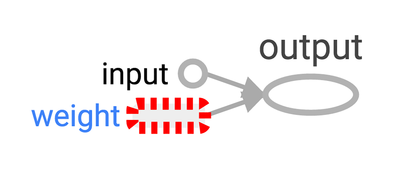
Up to this point, the graph has been simple, but it would already be nice to see it represented in a diagram. We’ll use TensorBoard to generate that diagram. TensorBoard reads the name field that is stored inside each operation (quite distinct from Python variable names). We can use these TensorFlow names and switch to more conventional Python variable names. Using tf.mul here is equivalent to our earlier use of just * for multiplication, but it lets us set the name for the operation.

>>> x = tf.constant(1.0, name='input')
>>> w = tf.Variable(0.8, name='weight')
>>> y = tf.mul(w, x, name='output')

TensorBoard works by looking at a directory of output created from TensorFlow sessions. We can write this output with a SummaryWriter, and if we do nothing aside from creating one with a graph, it will just write out that graph.

The first argument when creating the SummaryWriter is an output directory name, which will be created if it doesn’t exist.

>>> summary_writer = tf.train.SummaryWriter('log_simple_graph', sess.graph)

Now, at the command line, we can start up TensorBoard.

$ tensorboard --logdir=log_simple_graph

TensorBoard runs as a local web app, on port 6006. (“6006” is “goog” upside-down.) If you go in a browser to localhost:6006/#graphs you should see a diagram of the graph you created in TensorFlow, which looks something like Figure 2.

Making the neuron learn

Now that we’ve built our neuron, how does it learn? We set up an input value of 1.0. Let’s say the correct output value is zero. That is, we have a very simple “training set” of just one example with one feature, which has the value one, and one label, which is zero. We want the neuron to learn the function taking one to zero.

Currently, the system takes the input one and returns 0.8, which is not correct. We need a way to measure how wrong the system is. We’ll call that measure of wrongness the “loss” and give our system the goal of minimizing the loss. If the loss can be negative, then minimizing it could be silly, so let’s make the loss the square of the difference between the current output and the desired output.

>>> y_ = tf.constant(0.0)
>>> loss = (y - y_)**2

So far, nothing in the graph does any learning. For that, we need an optimizer. We’ll use a gradient descent optimizer so that we can update the weight based on the derivative of the loss. The optimizer takes a learning rate to moderate the size of the updates, which we’ll set at 0.025.

>>> optim = tf.train.GradientDescentOptimizer(learning_rate=0.025)

The optimizer is remarkably clever. It can automatically work out and apply the appropriate gradients through a whole network, carrying out the backward step for learning.

Let’s see what the gradient looks like for our simple example.

>>> grads_and_vars = optim.compute_gradients(loss)
>>> sess.run(tf.initialize_all_variables())
>>> sess.run(grads_and_vars[1][0])
## 1.6

Why is the value of the gradient 1.6? Our loss is error squared, and the derivative of that is two times the error. Currently the system says 0.8 instead of 0, so the error is 0.8, and two times 0.8 is 1.6. It’s working!

For more complex systems, it will be very nice indeed that TensorFlow calculates and then applies these gradients for us automatically.

Let’s apply the gradient, finishing the backpropagation.

>>> sess.run(optim.apply_gradients(grads_and_vars))
>>> sess.run(w)
## 0.75999999  # about 0.76

The weight decreased by 0.04 because the optimizer subtracted the gradient times the learning rate, 1.6 * 0.025, pushing the weight in the right direction.

Instead of hand-holding the optimizer like this, we can make one operation that calculates and applies the gradients: the train_step.

>>> train_step = tf.train.GradientDescentOptimizer(0.025).minimize(loss)
>>> for i in range(100):
>>>     sess.run(train_step)
>>> 
>>> sess.run(y)
## 0.0044996012

Running the training step many times, the weight and the output value are now very close to zero. The neuron has learned!

Training diagnostics in TensorBoard

We may be interested in what’s happening during training. Say we want to follow what our system is predicting at every training step. We could print from inside the training loop.

>>> sess.run(tf.initialize_all_variables())
>>> for i in range(100):
>>>     print('before step {}, y is {}'.format(i, sess.run(y)))
>>>     sess.run(train_step)
>>> 
## before step 0, y is 0.800000011921
## before step 1, y is 0.759999990463
## ...
## before step 98, y is 0.00524811353534
## before step 99, y is 0.00498570781201

This works, but there are some problems. It’s hard to understand a list of numbers. A plot would be better. And even with only one value to monitor, there’s too much output to read. We’re likely to want to monitor many things. It would be nice to record everything in some organized way.

Luckily, the same system that we used earlier to visualize the graph also has just the mechanisms we need.

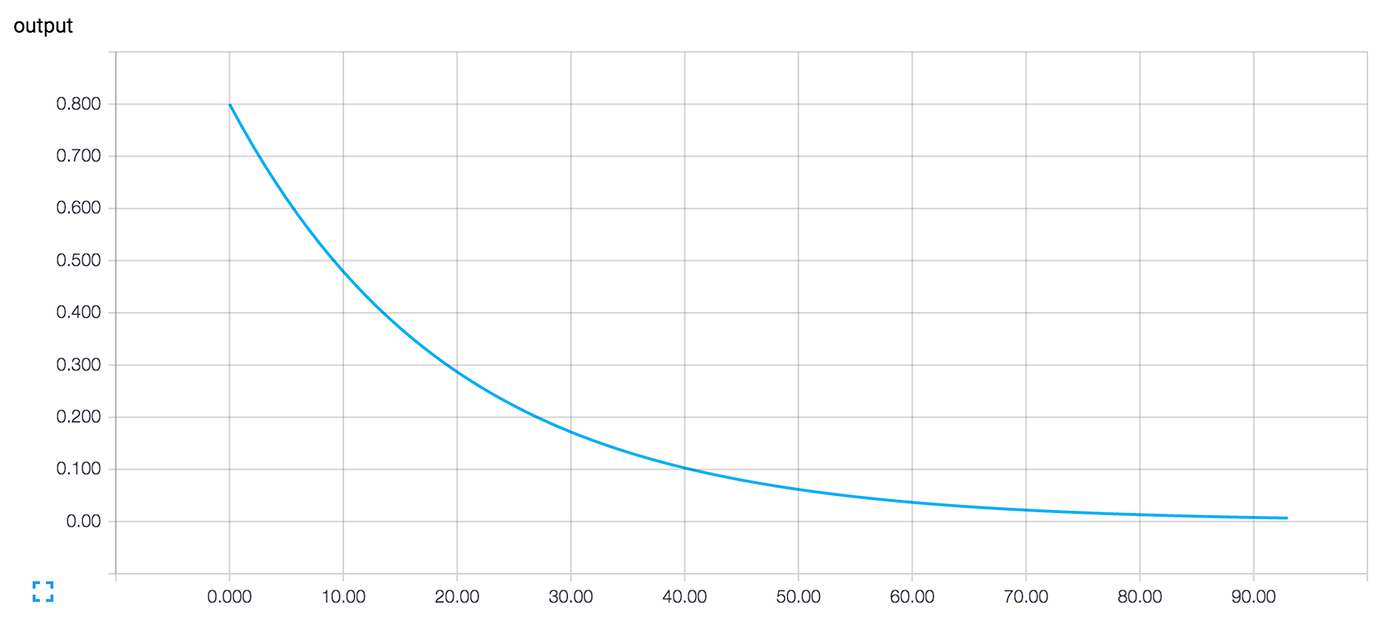
We instrument the computation graph by adding operations that summarize its state. Here, we’ll create an operation that reports the current value of y, the neuron’s current output.

>>> summary_y = tf.scalar_summary('output', y)

When you run a summary operation, it returns a string of protocol buffer text that can be written to a log directory with a SummaryWriter.

>>> summary_writer = tf.train.SummaryWriter('log_simple_stats')
>>> sess.run(tf.initialize_all_variables())
>>> for i in range(100):
>>>     summary_str = sess.run(summary_y)
>>>     summary_writer.add_summary(summary_str, i)
>>>     sess.run(train_step)
>>> 

Now after running tensorboard --logdir=log_simple_stats, you get an interactive plot at localhost:6006/#events (Figure 3).

Flowing onward

Here’s a final version of the code. It’s fairly minimal, with every part showing useful (and understandable) TensorFlow functionality.

import tensorflow as tf

x = tf.constant(1.0, name='input')
w = tf.Variable(0.8, name='weight')
y = tf.mul(w, x, name='output')
y_ = tf.constant(0.0, name='correct_value')
loss = tf.pow(y - y_, 2, name='loss')
train_step = tf.train.GradientDescentOptimizer(0.025).minimize(loss)

for value in [x, w, y, y_, loss]:
    tf.scalar_summary(value.op.name, value)

summaries = tf.merge_all_summaries()

sess = tf.Session()
summary_writer = tf.train.SummaryWriter('log_simple_stats', sess.graph)

sess.run(tf.initialize_all_variables())
for i in range(100):
    summary_writer.add_summary(sess.run(summaries), i)
    sess.run(train_step)

The example we just ran through is even simpler than the ones that inspired it in Michael Nielsen’s Neural Networks and Deep Learning. For myself, seeing details like these helps with understanding and building more complex systems that use and extend from simple building blocks. Part of the beauty of TensorFlow is how flexibly you can build complex systems from simpler components.

If you want to continue experimenting with TensorFlow, it might be fun to start making more interesting neurons, perhaps with different activation functions. You could train with more interesting data. You could add more neurons. You could add more layers. You could dive into more complex pre-built models, or spend more time with TensorFlow’s own tutorials and how-to guides. Go for it!