Shared nothing architectures: Giving Hadoop’s data processing frameworks scalability and fault tolerance

MapReduce Overview

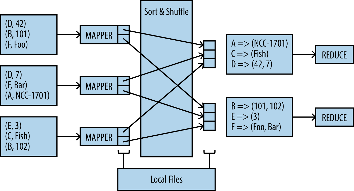
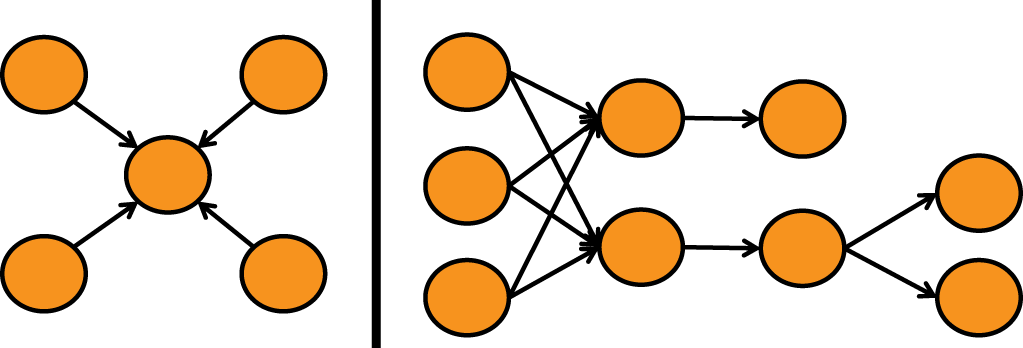
The MapReduce programming paradigm breaks processing into two basic phases: a map phase and a reduce phase. The input and output of each phase are key-value pairs.

The processes executing the map phase are called mappers. Mappers are Java processes (JVMs) that normally start up on nodes that also contain the data they will process. Data locality is an important principle of MapReduce; with large data sets, moving the processing to the servers that contain the data is much more efficient than moving the data across the network. An example of the types of processing typically performed in mappers are parsing, transformation, and filtering. When the mapper has processed the input data it will output a key-value pair to the next phase, the sort and shuffle.

In the sort and shuffle phase, data is sorted and partitioned. We will discuss the details of how this works later in the chapter. This partitioned and sorted data is sent over the network to reducer JVMs that read the data ordered and partitioned by the keys. When a reducer process gets these records, the reduce0 function can do any number of operations on the data, but most likely the reducer will write out some amount of the data or aggregate to a store like HDFS or HBase.

To summarize, there are two sets of JVMs. One gets data unsorted and the other gets data sorted and partitioned. There are many more parts to MapReduce that we will touch on in a minute, but Figure 1-1 shows what has been described so far.

The following are some typical characteristics of MapReduce processing:

• Mappers process input in key-value pairs and are only able to process a single pair at a time. The number of mappers is set by the framework, not the developer.

• Mappers pass key-value pairs as output to reducers, but can’t pass information to other mappers. Reducers can’t communicate with other reducers either.

• Mappers and reducers typically don’t use much memory and the JVM heap size is set relatively low.

• Each reducer typically, although not always, has a single output stream—by default a set of files named part-r-00000, part-r-00001, and so on, in a single HDFS directory.

• The output of the mapper and the reducer is written to disk. If the output of the reducer requires additional processing, the entire data set will be written to disk and then read again. This pattern is called synchronization barrier and is one of the major reasons MapReduce is considered inefficient for iterative processing of data.

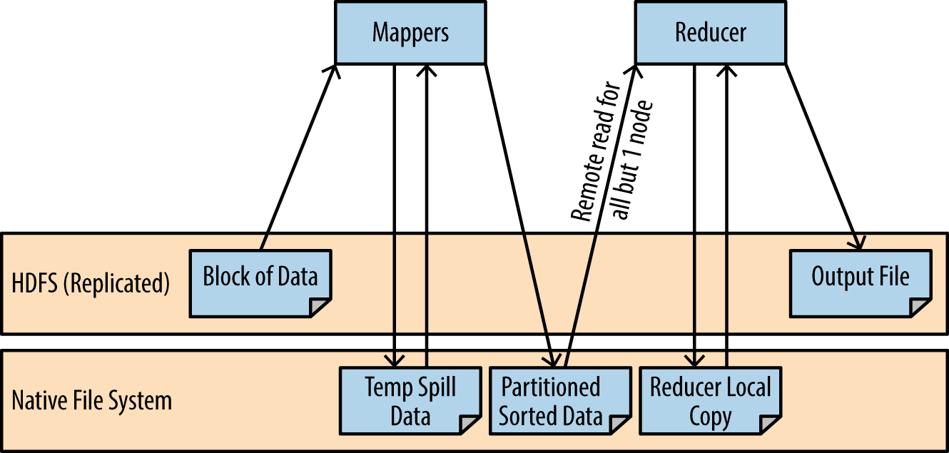
Before we go into the lower-level details of MapReduce, it is important to note that MapReduce has two major weaknesses that make it a poor option for iterative algorithms. The first is the startup time. Even if you are doing almost nothing in the MapReduce processing, there is a loss of 10—30 seconds just to startup cost. Second, MapReduce writes to disk frequently in order to facilitate fault tolerance. Later on in this chapter when we study Spark, we will learn that all this disk I/O isn’t required. Figure 1-2 illustrates how many times MapReduce reads and writes to disk during typical processing.

One of the things that makes MapReduce so powerful is the fact that it is made not just of map and reduce tasks, but rather multiple components working together. Each one of these components can be extended by the developer. Therefore, in order to make the most out of MapReduce, it is important to understand its basic building blocks in detail. In the next section we’ll start with a detailed look into the map phase in order to work toward this understanding.

There are a number of good references that provide more detail on MapReduce than we can go into here, including implementations of various algorithms. Some good resources are Hadoop: The Definitive Guide, Hadoop in Practice, and MapReduce Design Patterns by Donald Miner and Adam Shook (O’Reilly).

Map phase

Next, we provide a detailed overview of the major components involved in the map phase of a MapReduce job.

InputFormat

MapReduce jobs access their data through the InputFormat class. This class implements two important methods:

getSplits()

This method implements the logic of how input will be distributed between the map processes. The most commonly used Input Format is the TextInputFormat, which will generate an input split per block and give the location of the block to the map task. The framework will then execute a mapper for each of the splits. This is why developers usually assume the number of mappers in a MapReduce job is equal to the number of blocks in the data set it will process.

This method determines the number of map processes and the cluster nodes on which they will execute, but because it can be overridden by the developer of the MapReduce job, you have complete control over the way in which files are read. For example, the NMapInputFormat in the HBase code base allows you to directly set the number of mappers executing the job.

getReader()

This method provides a reader to the map task that allows it to access the data it will process. Because the developer can override this method, MapReduce can support any data type. As long as you can provide a method that reads the data into a writable object, you can process it with the MapReduce framework.

RecordReader

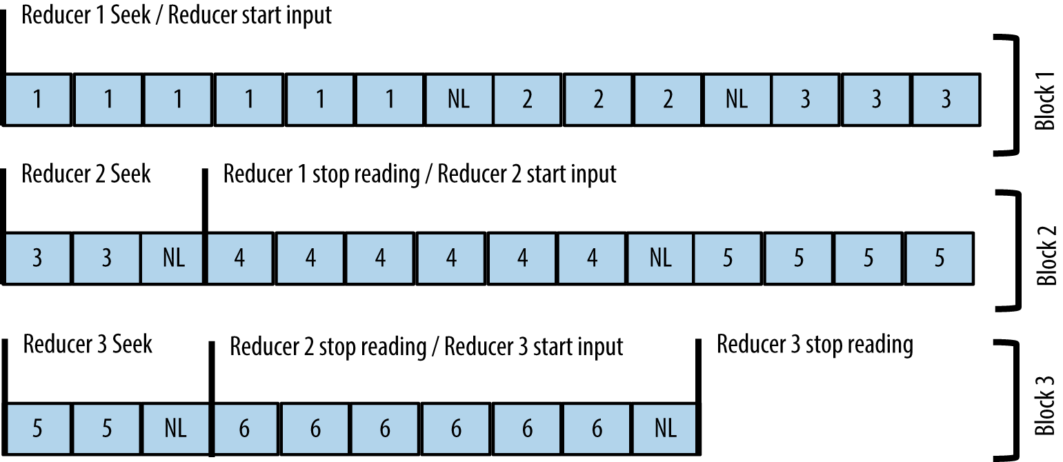
The RecordReader class reads the data blocks and returns key-value records to the map task. The implementation of most RecordReaders is surprisingly simple:
a RecordReader instance is initialized with the start position in the file for the block it needs to read and the URI of the file in HDFS. After seeking to the start position, each call to nextKeyValue() will find the next row delimiter and read the next record. This pattern is illustrated in Figure 1-3.

The MapReduce framework and other ecosystem projects provide RecordReader implementations for many file formats: text delimited, SequenceFile, Avro, Parquet, and more. There are even RecordReaders that don’t read any data—NMapInputFormat returns a NullWritable as the key and value to the mapper. This is to make sure the map() method gets called once.

Mapper.setup()

Before the map method of the map task gets called, the mapper’s setup() method is called once. This method is used by developers to initialize variables and file handles that will later get used in the map process. Very frequently the setup() method is used to retrieve values from the configuration object.

Every component in Hadoop is configured via a Configuration object, which contains key-value pairs and is passed to the map and reduce JVMs when the job is executed. The contents of this object can be found in job.xml. By default the Configuration object contains information regarding the cluster that every JVM requires for successful execution, such as the URI of the NameNode and the process coordinating the job (e.g., the JobTracker when Hadoop is running within the MapReduce v1 framework or the Application Manager when it’s running with YARN).

Values can be added to the Configuration object in the setup phase, before the map and reduce tasks are launched. After the job is executed, the mappers and reducers can access the Configuration object at any time to retrieve these values. Here is a simple example of a setup() method that gets a Configuration value to populate a member variable:

public String fooBar;
public final String FOO_BAR_CONF = "custom.foo.bar.conf";

@Override
public void setup(Context context) throws IOException {
  foobar = context.getConfiguration().get(FOO_BAR_CONF);
}

Note that anything you put in the Configuration object can be read through the JobTracker (in MapReduce v1) or Application Manager (in YARN). These processes have a web UI that is often left unsecured and readable to anyone with access to its URL, so we recommend against passing sensitive information such as passwords through the Configuration object. A better method is to pass the URI of a password file in HDFS, which can have proper access permissions. The map and reduce tasks can then read the content of the file and get the password if the user executing the MapReduce job has sufficient privileges.

Mapper.map

The map() method is the heart of the mapper. Even if you decide to use the defaults and not implement any other component of the map task, you will still need to implement a map() method. This method has three inputs: key, value, and a context. The key and value are provided by the RecordReader and contain the data that the map() method should process. The context is an object that provides common actions for a mapper: sending output to the reducer, reading values from the Configuration object, and incrementing counters to report on the progress of the map task.

When the map task writes to the reducer, the data it is writing is buffered and sorted. MapReduce will attempt to sort it in memory, with the available space defined by the io.sort.mb configuration parameter. If the memory buffer is too small, not all the output data can be sorted in memory. In this case the data is spilled to the local disk of the node where the map task is running and sorted on disk.

Partitioner

The partitioner implements the logic of how data is partitioned between the reducers. The default partitioner will simply take the key, hash it using a standard hash function, and divide by the number of reducers. The remainder will determine the target reducer for the record. This guarantees equal distribution of data between the reducers, which will help ensure that reducers can begin and end at the same time. But if there is any requirement for keeping certain values together for processing by the reducers, you will need to override the default and implement a custom partitioner.

One such example is a secondary sort. Suppose that you have a time series—for example, stock market pricing information. You may wish to have each reducer scan all the trades of a given stock ticker ordered by the time of the trade in order to look for correlations in pricing over time. In this case you will define the key as ticker-time. The default partitioner could send records belonging to the same stock ticker to different reducers, so you will also want to implement your own partitioner to make sure the ticker symbol is used for partitioning the records to reducers, but the timestamp is not used.

Here is a simple code example of how this type of partitioner method would be implemented:

public static class CustomPartitioner extends Partitioner<Text, Text> {
    @Override
    public int getPartition(Text key, Text value, int numPartitions) {
      String ticker = key.toString().substring(5);
      return ticker.hashCode() % numPartitions;
    }
  }

We simply extract the ticker symbol out of the key and use only the hash of this part for partitioning instead of the entire key.

Mapper.cleanup()

The cleanup() method is called after the map() method has executed for all records. This is a good place to close files and to do some last-minute reporting—for example, to write a message to the log with final status.

Combiner

Combiners in MapReduce can provide an easy method to reduce the amount of network traffic between the mappers and reducers. Let’s look at the famous word count example. In word count, the mapper takes each input line, splits it into individual words and writes out each word with “1” after it, to indicate current count, like the following:

• the => 1
• cat => 1
• and => 1
• the => 1
• hat => 1

If a combine() method is defined it can aggregate the values produced by the mapper. It executes locally on the same node where the mapper executes, so this aggregation reduces the output that is later sent through the network to the reducer. The reducer will still have to aggregate the results from different mappers, but this will be over significantly smaller data sets. It is important to remember that you have no control on whether the combiner will execute. Therefore, the output of the combiner has to be identical in format to the output of the mapper, because the reducer will have to process either of them. Also note that the combiner executes after the output of the mapper is already sorted, so you can assume that the input of the combiner is sorted.

In our example, this would be the output of a combiner:

• and => 1
• cat => 1
• hat => 1
• the => 2

Example for MapReduce

Of all the approaches to data processing in Hadoop that will be included in this chapter, MapReduce requires the most code by far. As verbose as this example will seem, if we included every part of MapReduce here, it would easily be another 20 pages. We will look at a very simple example: joining and filtering the two data sets shown in Figure 1-4.

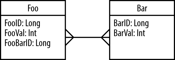
The data processing requirements in this example include:

• Join Foo to Bar by FooBarId and BarId.

• Filter Foo and remove all records where FooVal is greater than a user-defined value, fooValueMaxFilter.

• Filter the joined table and remove all records where the sum of FooVal and BarVal is greater than another user parameter, joinValueMaxFilter.

• Use counters to track the number of rows we removed.

MapReduce jobs always start by creating a Job instance and executing it. Here is an example of how this is done:

  public int run(String[] args) throws Exception {
    String inputFoo = args[0];
    String inputBar = args[1];
    String output = args[2];
    String fooValueMaxFilter = args[3];
    String joinValueMaxFilter = args[4];
    int numberOfReducers = Integer.parseInt(args[5]);

    Job job = Job.getInstance();	

    job.setJarByClass(JoinFilterExampleMRJob.class);
    job.setJobName("JoinFilterExampleMRJob");	

    Configuration config = job.getConfiguration();
    config.set(FOO_TABLE_CONF, inputFoo);	
    config.set(BAR_TABLE_CONF, inputBar);
    config.set(FOO_VAL_MAX_CONF, fooValueMaxFilter);
    config.set(JOIN_VAL_MAX_CONF, joinValueMaxFilter);

    job.setInputFormatClass(TextInputFormat.class);
    TextInputFormat.addInputPath(job, new Path(inputFoo));	
    TextInputFormat.addInputPath(job, new Path(inputBar));
    job.setOutputFormatClass(TextOutputFormat.class);
    TextOutputFormat.setOutputPath(job, new Path(output));

    job.setMapperClass(JoinFilterMapper.class);	
    job.setReducerClass(JoinFilterReducer.class);
    job.setPartitionerClass(JoinFilterPartitioner.class);
    job.setOutputKeyClass(NullWritable.class);
    job.setOutputValueClass(Text.class);
    job.setMapOutputKeyClass(Text.class);
    job.setMapOutputValueClass(Text.class);

    job.setNumReduceTasks(numberOfReducers);	

    job.waitForCompletion(true);	
    return 0;
  }

Let’s drill down into the job setup code:

This is the constructor of the Job object that will hold all the information needed for the execution of our MapReduce job.

While not mandatory, it is a good practice to name the job so it will be easy to find in various logs or web UIs.

As we discussed, when setting up the job, you can create a Configuration object with values that will be available to all map and reduce tasks. Here we add the values that will be used for filtering the records, so they are defined by the user as arguments when the job is executed, not hardcoded into the map and reduce tasks.

Here we are setting the input and output directories. There can be multiple input paths, and they can be either files or entire directories. But unless a special output format is used, there is only one output path and it must be a directory, so each reducer can create its own output file in that directory.

This is where we configure the classes that will be used in this job: mapper, reducer, partitioner, and the input and output formats. In our example we only need a mapper, reducer, and partitioner. We will soon show the code used to implement each of those. Note that for the output format we use Text as the value output, but NullWritable as the key output. This is because we are only interested in the values for the final output. The keys will simply be ignored and not written to the reducer output files.

While the number of mappers is controlled by the input format, we have to configure the number of reducers directly. If the number of reducers is set to 0, we would get a map-only job. The default number of reducers is defined at the cluster level, but is typically overridden by the developers of specific jobs because they are more familiar with the size of the data involved and how it is partitioned.

Finally, we fire off the configured MapReduce job to the cluster and wait for its success or failure.

Now let’s look at the mapper:

public class JoinFilterMapper extends
  Mapper<LongWritable, Text, Text, Text> {

  boolean isFooBlock = false;
  int fooValFilter;

  public static final int FOO_ID_INX = 0;
  public static final int FOO_VALUE_INX = 1;
  public static final int FOO_BAR_ID_INX = 2;
  public static final int BAR_ID_INX = 0;
  public static final int BAR_VALUE_INX = 1;

  Text newKey = new Text();
  Text newValue = new Text();

  @Override
  public void setup(Context context) {


    Configuration config = context.getConfiguration();	
    fooValFilter = config.getInt(JoinFilterExampleMRJob.FOO_VAL_MAX_CONF, -1);


    String fooRootPath =
      config.get(JoinFilterExampleMRJob.FOO_TABLE_CONF); 
    FileSplit split = (FileSplit) context.getInputSplit();
    if (split.getPath().toString().contains(fooRootPath)) {
      isFooBlock = true;
    }
  }

  @Override
  public void map(LongWritable key, Text value, Context context)
      throws IOException, InterruptedException {

    String[] cells = StringUtils.split(value.toString(), "|");


    if (isFooBlock) {	
      int fooValue = Integer.parseInt(cells[FOO_VALUE_INX]);

      if (fooValue <= fooValFilter) {	
        newKey.set(cells[FOO_BAR_ID_INX] + "|"
            + JoinFilterExampleMRJob.FOO_SORT_FLAG);
        newValue.set(cells[FOO_ID_INX] + "|" + cells[FOO_VALUE_INX]);
        context.write(newKey, newValue);
      } else {
        context.getCounter("Custom", "FooValueFiltered").increment(1); 
      }
    } else {
      newKey.set(cells[BAR_ID_INX] + "|" +
             JoinFilterExampleMRJob.BAR_SORT_FLAG);	
      newValue.set(cells[BAR_VALUE_INX]);
      context.write(newKey, newValue);
    }
  }
}

As we discussed, the mapper’s setup() method is used to read predefined values from the Configuration object. Here we are getting the fooValMax filter value that we will use later in the map() method for filtering.

Each map task will read data from a file block that belongs either to the Foo or Bar data sets. We need to be able to tell which is which, so we can filter only the data from Foo tables and so we can add this information to the output key—it will be used by the reducer for joining the data sets. In this section of the code, the setup() method identifies which block we are processing in this task. Later, in the map() method, we will use this value to separate the logic for processing the Foo and Bar data sets.

This is where we use the block identifier we defined earlier.

And here we use the fooValMax value for filtering.

The last thing to point out here is the method to increment a counter in MapReduce. A counter has a group and counter name, and both can be set and incremented by the map and reduce tasks. They are reported at the end of the job and are also tracked by the various UIs while the job is executing, so it is a good way to give users feedback on the job progress, as well as give the developers useful information for debugging and troubleshooting.

Note how we set the output key: first there is the value used to join the data sets, followed by “|” and then a flag marking the record with A if it arrived from the Bar data set and B if it arrived from Foo. This means that when the reducer receives a key and an array of values to join, the values from the Bar data set will appear first (since keys are sorted). To perform the join we will only have to store the Bar data set in memory until the Foo values start arriving. Without the flag to assist in sorting the values, we will need to store the entire data set in memory when joining.

Now let’s look into the partitioner. We need to implement a customer partitioner because we are using a multipart key that contains the join key plus the sort flag. We need to partition only by ID, so both records with the same join key will end up in the same reducer regardless of whether they originally arrived from the data set Foo or Bar. This is essential for joining them because a single reducer will need to join all values with the same key. To do this, we need only partition on the ID and entire composite key as shown:

public class JoinFilterPartitioner extends Partitioner<Text, Text>{

  @Override
  public int getPartition(Text key, Text value, int numberOfReducers) {
    String keyStr = key.toString();

    String pk = keyStr.substring(0, keyStr.length() - 2);

    return Math.abs(pk.hashCode() % numberOfReducers);
  }

}

In the partitioner we get the join key out of the key in the map output and apply the partitioning method using this part of the key only, as we discussed previously.

Next we’ll look at the reducer and how it joins the two data sets:

public class JoinFilterReducer extends Reducer<Text, Text, NullWritable, Text> {

  int joinValFilter;
  String currentBarId = "";
  List<Integer> barBufferList = new ArrayList<Integer>();

  Text newValue = new Text();

  @Override
  public void setup(Context context) {
    Configuration config = context.getConfiguration();
    joinValFilter = config.getInt(JoinFilterExampleMRJob.JOIN_VAL_MAX_CONF, -1);
  }

  @Override
  public void reduce(Text key, Iterable<Text> values, Context context)
      throws IOException, InterruptedException {

    String keyString = key.toString();
    String barId = keyString.substring(0, keyString.length() - 2);
    String sortFlag = keyString.substring(keyString.length() - 1);

    if (!currentBarId.equals(barId)) {
      barBufferList.clear();
      currentBarId = barId;
    }

    if (sortFlag.equals(JoinFilterExampleMRJob.BAR_SORT_FLAG)) { 
      for (Text value : values) {
        barBufferList.add(Integer.parseInt(value.toString())); 
      }
    } else {
      if (barBufferList.size() > 0) {
        for (Text value : values) {
          for (Integer barValue : barBufferList) { 

            String[] fooCells = StringUtils.split(value.toString(), "|");

            int fooValue = Integer.parseInt(fooCells[1]);
            int sumValue = barValue + fooValue;

            if (sumValue < joinValFilter) {

              newValue.set(fooCells[0] + "|" + barId + "|" + sumValue);
              context.write(NullWritable.get(), newValue);
            } else {
              context.getCounter("custom", "joinValueFiltered").increment(1);
            }
          }
        }
      } else {
        System.out.println("Matching with nothing");
      }
    }
  }
}

Because we used a flag to assist in sorting, we are getting all the records from the Bar data set for a given join key first.

As we receive them, we store all the Bar records in a list in memory.

As we process the Foo records, we’ll loop through the cached Bar records to execute the join. This is a simple implementation of a nested-loops join.

When to Use MapReduce

As you can see from the example, MapReduce is a very low-level framework. The developer is responsible for very minute details of operation, and there is a significant amount of setup and boilerplate code. Because of this MapReduce code typically has more bugs and higher costs of maintenance.

However, there is a subset of problems, such as file compaction,¹ distributed file-copy, or row-level data validation, which translates to MapReduce quite naturally. At other times, code written in MapReduce can take advantage of properties of the input data to improve performance—for example, if we know the input files are sorted, we can use MapReduce to optimize merging of data sets in ways that higher-level abstractions can’t.

We recommend MapReduce for experienced Java developers who are comfortable with the MapReduce programming paradigm, especially for problems that translate to MapReduce naturally or where detailed control of the execution has significant advantages.

Spark Overview

Spark is different from MapReduce in several important ways.

DAG Model

Looking back at MapReduce you only had two processing phases: map and/or reduce. With the MapReduce framework, it is only possible to build complete applications by stringing together sets of map and reduce tasks. These complex chains of tasks are known as directed acyclic graphs, or DAGs, illustrated in Figure 1-5.

DAGs contain series of actions connected to each other in a workflow. In the case of MapReduce, the DAG is a series of map and reduce tasks used to implement the application. The use of DAGs to define Hadoop applications is not new—MapReduce developers implemented these, and they are used within all high-level abstractions that use MapReduce. Oozie even allows users to define these workflows of MapReduce tasks in XML and use an orchestration framework to monitor their execution.

What Spark adds is the fact that the engine itself creates those complex chains of steps from the application’s logic, rather than the DAG being an abstraction added externally to the model. This allows developers to express complex algorithms and data processing pipelines within the same job and allows the framework to optimize the job as a whole, leading to improved performance.

For more on Spark, see the Apache Spark site. There are still relatively few texts available on Spark, but Learning Spark by Holden Karau, et al. (O’Reilly) will provide a comprehensive introduction to Spark. For more advanced Spark usage, see the Advanced Analytics with Spark by Sandy Ryza, et al. (O’Reilly).

Overview of Spark Components

Before we get to the example, it is important to go over the different parts of Spark at a high level. Figure 1-6 shows the major Spark components.

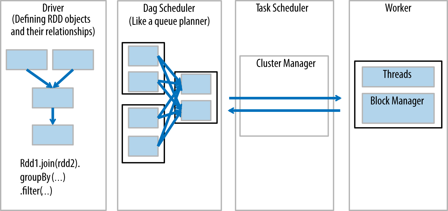
Let’s discuss the components in this diagram from left to right:

• The driver is the code that includes the “main” function and defines the resilient distributed datasets (RDDs) and their transformations. RDDs are the main data structures we will use in our Spark programs, and will be discussed in more detail in the next section.

• Parallel operations on the RDDs are sent to the DAG scheduler, which will optimize the code and arrive at an efficient DAG that represents the data processing steps in the application.

• The resulting DAG is sent to the cluster manager. The cluster manager has information about the workers, assigned threads, and location of data blocks and is responsible for assigning specific processing tasks to workers. The cluster manager is also the service that handles DAG play-back in the case of worker failure. As we explained earlier, the cluster manager can be YARN, Mesos, or Spark’s cluster manager.

• The worker receives units of work and data to manage. The worker executes its specific task without knowledge of the entire DAG, and its results are sent back to the driver application.

Basic Spark Concepts

Before we go into the code for our filter-join-filter example, let’s talk about the main components of writing applications in Spark.

Resilient Distributed Datasets

RDDs are collections of serializable elements, and such a collection may be partitioned, in which case it is stored on multiple nodes. An RDD may reside in memory or on disk. Spark uses RDDs to reduce I/O and maintain the processed data set in memory, while still tolerating node failures without having to restart the entire job.

RDDs are typically created from a Hadoop input format (a file on HDFS, for example), or from transformations applied on existing RDDs. When creating an RDD from an input format, Spark determines the number of partitions by the input format, very similar to the way splits are determined in MapReduce jobs. When RDDs are transformed, it is possible to shuffle the data and repartition it to any number of partitions.

RDDs store their lineage—the set of transformations that was used to create the current state, starting from the first input format that was used to create the RDD. If the data is lost, Spark will replay the lineage to rebuild the lost RDDs so the job can continue.

Figure 1-7 is a common image used to illustrate a DAG in spark. The inner boxes are RDD partitions; the next layer is an RDD and single chained operation.

Now let’s say we lose the partition denoted by the black box in Figure 1-8. Spark would replay the “Good Replay” boxes and the “Lost Block” boxes to get the data needed to execute the final step.

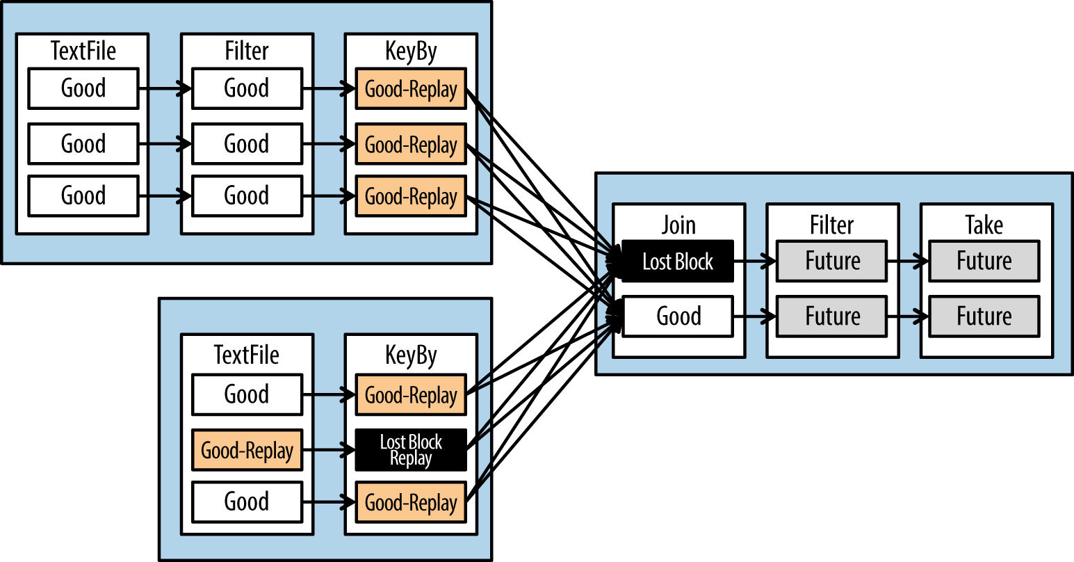
Note that there are multiple types of RDDs, and not all transformations are possible on every RDD. For example, you can’t join an RDD that doesn’t contain a key-value pair.

Benefits of Using Spark

Next, we’ll outline several of the advantages of using Spark.

Spark Example

With the introduction behind us, let’s look at the first code example. It uses the same data sets as the example in the MapReduce section and processes the data in the same way:

var fooTable = sc.textFile("foo")                                   

var barTable = sc.textFile("bar")

var fooSplit = fooTable.map(line => line.split("\\|"))              

var fooFiltered = fooSplit.filter(cells => cells(1).toInt <= 500)   

var fooKeyed = fooFiltered.keyBy(cells => cells(2))                 

var barSplit = barTable.map(line => line.split("\\|"))              

var barKeyed = barSplit.keyBy(cells => cells(0))

var joinedValues = fooKeyed.join(barKeyed)                          

var joinedFiltered =                                                
joinedValues.filter(joinedVal =>
  joinedVal._2._1(1).toInt + joinedVal._2._2(1).toInt <= 1000)

joinedFiltered.take(100)                                            

This code will do the following:

Load Foo and Bar data sets into two RDDs.

Split each row of Foo into a collection of separate cells.

Filter the split Foo data set and keep only the elements where the second column is smaller than 500.

Convert the results into key-value pairs using the ID column as the key.

Split the columns in Bar in the same way we split Foo and again convert into key-value pairs with the ID as the key.

Join Bar and Foo.

Filter the joined results. The filter() function here takes the value of the joinedVal RDD, which contains a pair of a Foo and a Bar row. We take the first column from each row and check if their sum is lower than 1,000.

Show the first 100 results. Note that this is the only action in the code, so the entire chain of transformations we defined here will only be triggered at this point.

This example is already pretty succinct, but it can be implemented in even fewer lines of code:

//short version
var fooTable = sc.textFile("foo")
  .map(line => line.split("\\|"))
  .filter(cells => cells(1).toInt <= 500)
  .keyBy(cells => cells(2))

var barTable = sc.textFile("bar")
  .map(line => line.split("\\|"))
  .keyBy(cells => cells(0))

var joinedFiltered = fooTable.join(barTable)
  .filter(joinedVal =>
    joinedVal._2._1(1).toInt + joinedVal._2._2(1).toInt <= 1000)

joinedFiltered.take(100)

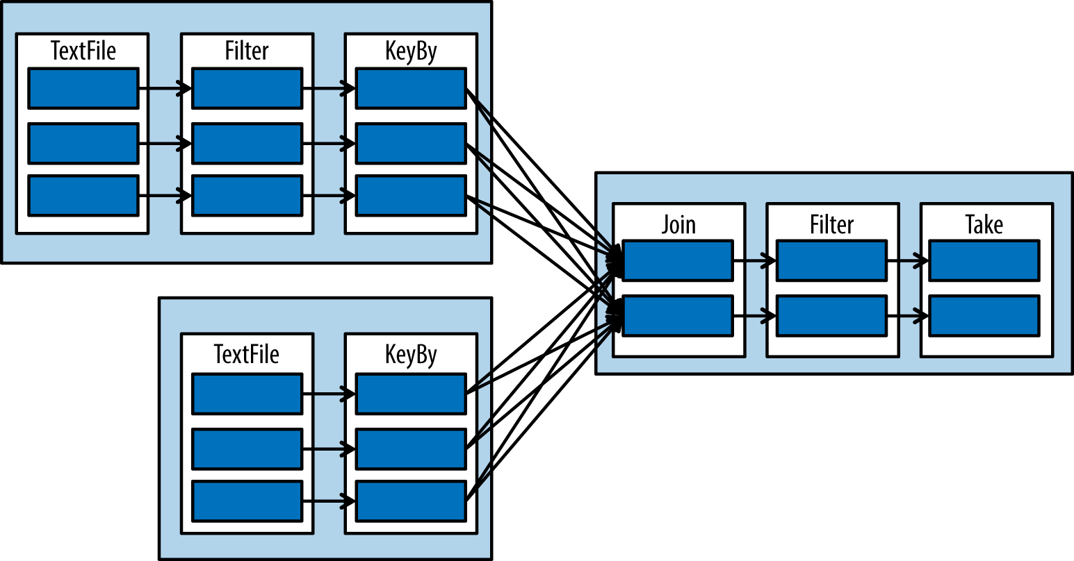
The execution plan this will produce looks like Figure 1-9.

When to Use Spark

While Spark is a fairly new framework at the moment, it is easy to use, extendable, highly supported, well designed, and fast. We see it rapidly increasing in popularity, and with good reason. Spark still has many rough edges, but as the framework matures and more developers learn to use it, we expect Spark to eclipse MapReduce for most functionality. Spark is already the best choice for machine-learning applications because of its ability to perform iterative operations on data cached in memory.

In addition to replacing MapReduce, Spark offers SQL, graph processing, and streaming frameworks. These projects are even less mature than Spark, and it remains to be seen how much adoption they will have and whether they will become reliable parts of the Hadoop ecosystem.

Pig

Pig is one of the oldest and most widely used abstractions over MapReduce in the Hadoop ecosystem. It was developed at Yahoo, and released to Apache in 2007.

Pig users write queries in a Pig-specific workflow language called Pig Latin, which gets compiled for execution by an underlying execution engine such as MapReduce. The Pig Latin scripts are first compiled into a logical plan and then into a physical plan. This physical plan is what gets executed by the underlying engine (e.g., MapReduce, Tez, or Spark). Due to Pig’s distinction between the logical and physical plan for a given query, only the physical plan changes when you use a different execution engine.

For more details on Pig, see the Apache Pig site or Programming Pig by Alan Gates (O’Reilly).

Pig Example

As you can see in this example, Pig Latin is fairly simple and self-expressive. As you review the code, you might note that it’s close to Spark in spirit:

fooOriginal = LOAD 'foo/foo.txt' USING PigStorage('|')
    AS (fooId:long, fooVal:int, barId:long);

fooFiltered = FILTER fooOriginal BY (fooVal <= 500);

barOriginal = LOAD 'bar/bar.txt' USING PigStorage('|')
   AS (barId:long, barVal:int);

joinedValues = JOIN fooFiltered by barId, barOriginal by barId;

joinedFiltered = FILTER joinedValues BY (fooVal + barVal <= 500);

STORE joinedFiltered INTO 'pig/out' USING PigStorage ('|');

Note the following in the preceding script:

Data container

This refers to identifiers like fooOriginal and fooFiltered that represent a data set. These are referred to as relations in Pig, and they are conceptually similar to the notion of RDDs in Spark (even though the actual persistence semantics of RDDs are very different). Speaking a little more about terminology, a relation is a bag, where a bag is a collection of tuples. A tuple is a collection of values/objects, which themselves could be bags, which could contain bags of more tuples, which could contain bags, and so on.

Transformation functions

This refers to operators like FILTER and JOIN that can transform relations. Again, logically just like Spark, these transformation functions do not force an action immediately. No execution is done until the STORE command is called, and nothing is done until the saveToTextFile is called.

Field definitions

Unlike in Spark, fields and their data types are called out (e.g., fooId:long). This makes dealing with field data easier and allows for other external tools to track lineage at a field level.

No Java

There are no commands for importing classes or objects in the preceding example. In some ways, you are limited by the dialect of Pig Latin, but in other ways, you get rid of the additional complexity of a programming language API to run your processing jobs. If you’d like a programming interface to your processing jobs, you will find later sections on Crunch and Cascading useful.

Pig also offers insight into its plan for running a job when issued a command like Explain JoinedFiltered from the previous example. Here is the output from our filter-join-filter job:

#--------------------------------------------------
# MapReduce Plan
#--------------------------------------------------
MapReduce node scope-43
Map Plan
Union[tuple] - scope-44
|
|---joinedValues: Local Rearrange[tuple]{long}(false) - scope-27
|   |   |
|   |   Project[long][2] - scope-28
|   |
|   |---fooFiltered: Filter[bag] - scope-11
|       |   |
|       |   Less Than or Equal[boolean] - scope-14
|       |   |
|       |   |---Project[int][1] - scope-12
|       |   |
|       |   |---Constant(500) - scope-13
|       |
|       |---fooOriginal: New For Each(false,false,false)[bag] - scope-10
|           |   |
|           |   Cast[long] - scope-2
|           |   |
|           |   |---Project[bytearray][0] - scope-1
|           |   |
|           |   Cast[int] - scope-5
|           |   |
|           |   |---Project[bytearray][1] - scope-4
|           |   |
|           |   Cast[long] - scope-8
|           |   |
|           |   |---Project[bytearray][2] - scope-7
|           |
|           |---fooOriginal: Load(hdfs://localhost:8020/foo/foo.txt:\
PigStorage('|')) - scope-0
|
|---joinedValues: Local Rearrange[tuple]{long}(false) - scope-29
    |   |
    |   Project[long][0] - scope-30
    |
    |---barOriginal: New For Each(false,false)[bag] - scope-22
        |   |
        |   Cast[long] - scope-17
        |   |
        |   |---Project[bytearray][0] - scope-16
        |   |
        |   Cast[int] - scope-20
        |   |
        |   |---Project[bytearray][1] - scope-19
        |
        |---barOriginal: Load(hdfs://localhost:8020/bar/bar.txt:\
PigStorage('|')) - scope-15--------
Reduce Plan
joinedFiltered: Store(fakefile:org.apache.pig.builtin.PigStorage) - scope-40
|
|---joinedFiltered: Filter[bag] - scope-34
    |   |
    |   Less Than or Equal[boolean] - scope-39
    |   |
    |   |---Add[int] - scope-37
    |   |   |
    |   |   |---Project[int][1] - scope-35
    |   |   |
    |   |   |---Project[int][4] - scope-36
    |   |
    |   |---Constant(500) - scope-38
    |
    |---POJoinPackage(true,true)[tuple] - scope-45--------
Global sort: false

From the explain plan, you can see that there is one MapReduce job just like in our MapReduce implementation, and we also see that Pig performs the filtering in the same places we did it in the MapReduce code. Consequently, at the core, the Pig code will be about the same speed as our MapReduce code. In fact, it may be faster because it stores the values in their native types, whereas in MapReduce we convert them back and forth to strings.

When to Use Pig

To wrap up our discussion of Pig, here is a list of reasons that make Pig a good choice for processing data on Hadoop:

• Pig Latin is very easy to read and understand.

• A lot of the complexity of MapReduce is removed.

• A Pig Latin script is very small compared to the size (in terms of number of lines and effort) of an equivalent MapReduce job. This makes the cost of maintaining Pig Latin scripts much lower than MapReduce jobs.

• No code compilation is needed. Pig Latin scripts can be run directly in the Pig console.

• Pig provides great tools to figure out what it is going on under the hood. You can use DESCRIBE joinedFiltered; to figure out what data types are in the collection and use Explain joinedFiltered; to figure out the MapReduce execution plan that Pig will use to get the results.

The biggest downside to Pig is the need to come up to speed on a new language—the concepts related to bags, tuples, and relations can present a learning curve for many developers.

Crunch Example

The next example is a Crunch program that will execute our filter-join-filter use case. You will notice the main body of logic is in the run() method. Outside the run() method are all the definitions of the business logic that will fire at different points in the pipeline. This is similar to the way this would be implemented with Java in Spark, and offers a nice separation of workflow and business logic:

public class JoinFilterExampleCrunch implements Tool {

  public static final int FOO_ID_INX = 0;
  public static final int FOO_VALUE_INX = 1;
  public static final int FOO_BAR_ID_INX = 2;

  public static final int BAR_ID_INX = 0;
  public static final int BAR_VALUE_INX = 1;

  public static void main(String[] args) throws Exception {
    ToolRunner.run(new Configuration(), new JoinFilterExampleCrunch(), args);
  }

  Configuration config;

  public Configuration getConf() {

    return config;
  }

  public void setConf(Configuration config) {
    this.config = config;

  }

  public int run(String[] args) throws Exception {

    String fooInputPath = args[0];
    String barInputPath = args[1];
    String outputPath = args[2];
    int fooValMax = Integer.parseInt(args[3]);
    int joinValMax = Integer.parseInt(args[4]);
    int numberOfReducers = Integer.parseInt(args[5]);

    Pipeline pipeline =
      new MRPipeline(JoinFilterExampleCrunch.class, getConf()); 

    PCollection<String> fooLines = pipeline.readTextFile(fooInputPath);  
    PCollection<String> barLines = pipeline.readTextFile(barInputPath);

    PTable<Long, Pair<Long, Integer>> fooTable = fooLines.parallelDo(  
        new FooIndicatorFn(),
        Avros.tableOf(Avros.longs(),
        Avros.pairs(Writables.longs(), Writables.ints())));

    fooTable = fooTable.filter(new FooFilter(fooValMax));  

    PTable<Long, Integer> barTable = barLines.parallelDo(new BarIndicatorFn(),
        Avros.tableOf(Avros.longs(), Avros.ints()));

    DefaultJoinStrategy<Long, Pair<Long, Integer>, Integer> joinStrategy =   
        new DefaultJoinStrategy
          <Long, Pair<Long, Integer>, Integer>
          (numberOfReducers);

    PTable<Long, Pair<Pair<Long, Integer>, Integer>> joinedTable =
      joinStrategy 
        .join(fooTable, barTable, JoinType.INNER_JOIN);

    PTable<Long, Pair<Pair<Long, Integer>, Integer>> filteredTable =
        joinedTable.filter(new JoinFilter(joinValMax));

    filteredTable.write(At.textFile(outputPath), WriteMode.OVERWRITE); 

    PipelineResult result = pipeline.done();

    return result.succeeded() ? 0 : 1;
  }

  public static class FooIndicatorFn extend
      MapFn<String, Pair<Long, Pair<Long, Integer>>> {

    private static final long serialVersionUID = 1L;

    @Override
    public Pair<Long, Pair<Long, Integer>> map(String input) {
      String[] cells = StringUtils.split(input.toString(), "|");

      Pair<Long, Integer> valuePair = new Pair<Long, Integer>(
          Long.parseLong(cells[FOO_ID_INX]),
          Integer.parseInt(cells[FOO_VALUE_INX]));

      return new Pair<Long, Pair<Long, Integer>>(
          Long.parseLong(cells[FOO_BAR_ID_INX]), valuePair);
    }
  }

  public static class FooIndicatorFn extends
      MapFn<String, Pair<Long, Pair<Long, Integer>>> {

    private static final long serialVersionUID = 1L;

    @Override
    public Pair<Long, Pair<Long, Integer>> map(String input) {
      String[] cells = StringUtils.split(input.toString(), "|");

      Pair<Long, Integer> valuePair = new Pair<Long, Integer>(
          Long.parseLong(cells[FOO_ID_INX]),
          Integer.parseInt(cells[FOO_VALUE_INX]));

      return new Pair<Long, Pair<Long, Integer>>(
          Long.parseLong(cells[FOO_BAR_ID_INX]), valuePair);
    }
  }

  public static class FooFilter extends
      FilterFn<Pair<Long, Pair<Long, Integer>>> {

    private static final long serialVersionUID = 1L;

    int fooValMax;

    FooFilter(int fooValMax) {
      this.fooValMax = fooValMax;
    }

    @Override
    public boolean accept(Pair<Long, Pair<Long, Integer>> input) {
      return input.second().second() <= fooValMax;
    }
  }

  public static class FooFilter extends
      FilterFn<Pair<Long, Pair<Long, Integer>>> {

    private static final long serialVersionUID = 1L;

    int fooValMax;

    FooFilter(int fooValMax) {
      this.fooValMax = fooValMax;
    }

    @Override
    public boolean accept(Pair<Long, Pair<Long, Integer>> input) {
      return input.second().second() <= fooValMax;
    }
  }

  public static class BarIndicatorFn extends MapFn<String, Pair<Long, Integer>> {

    private static final long serialVersionUID = 1L;

    @Override
    public Pair<Long, Integer> map(String input) {
      String[] cells = StringUtils.split(input.toString(), "|");

      return new Pair<Long, Integer>(Long.parseLong(cells[BAR_ID_INX]),
          Integer.parseInt(cells[BAR_VALUE_INX]));
    }
  }

  public static class JoinFilter extends
      FilterFn<Pair<Long, Pair<Pair<Long, Integer>, Integer>>> {

    private static final long serialVersionUID = 1L;

    int joinValMax;

    JoinFilter(int joinValMax) {
      this.joinValMax = joinValMax;
    }

    @Override
    public boolean accept(Pair<Long,
                     Pair<Pair<Long, Integer>,
                     Integer>> input) {

      return input.second().first().second() +
          input.second().second() <= joinValMax;
    }

  }
}

Let’s walk through this code to see what’s going on:

We kick things off by creating an instance of MRPipeline, passing in a configuration object. Note that by selecting the MRPipeline class we’re using MapReduce as the underlying engine. Alternatively, we could switch this out for another engine such as Spark.

These two lines are where we add inputs to our newly created pipeline, sorting them in a PCollection. This idea is very in line with what we saw from Spark with RDDs. Think of this as an immutable distributed collection, and any operations on it will also most likely have to be distributed. Also like Spark, a PCollection may not always be physical; in other words, it might be stored in memory or on disk.

Here we see our first parallelDo, which is like an RDD map() function in Spark. It will run over all the items in the PCollection in a distributed way and return either another PCollection, or in this case a PTable. Note this calls a method called FooIndicatorFn(). We will go into this method in a minute, but for now just know it gets called for each record in a distributed manner across the data set. The rest of the parameters tell Crunch what we intend to return in terms of a new PTable. The PTable is different from a PCollection in that we now need a key and value—this will help when we start joining.

Generate a new PTable via a distributed filter.

Define a join strategy for the join that will happen on the next line. We’ll be using the DefaultJoinStrategy, but there are many other options, like BloomFilterJoinStrategy, MapsideJoinStrategy, and ShardedJoinStrategy. It’s always important to understand your data set before selecting a join strategy.

Here is our first example of a join operation. We’re using our newly created join strategy, the input PTables, and an inner or outer definition.

Finally, we write out our data to disk. Remember that this is still a distributed write, so it’s highly likely that you will see many files in the output directory, one file per thread.

When to Use Crunch

Given its similarities to Spark, is it reasonable to assume that Crunch will eventually be replaced by Spark for most developers? This will likely vary based on several factors. If you’re using Crunch over Spark, you get the benefits of an abstraction, while being shielded from the potential for something replacing Spark as the underlying engine.

However, these benefits of abstraction come at a cost. To truly be good at an abstraction you have to understand the underlying engine as well, so now you will have to learn Spark and Crunch. Also, there may be new functionality in Spark that hasn’t reached Crunch and thus will be inaccessible to you until Crunch is updated.

Most likely, some developers who are currently using Crunch will continue to use it. But in addition to competition from the other abstractions—like Pig, and to a lesser extent Cascading—just like MapReduce Crunch also has competition from the underlying execution engine. Despite this, Crunch may be a good choice if you like Java, and you like the idea of an abstraction layer between you and the underlying execution engine.

Cascading Example

The following example is an implementation of the filter-join-filter code in Cascading. When you’re first reading this code it may feel complex and different from Crunch and Spark, but on further examination you will see that they are very much alike:

public class JoinFilterExampleCascading {
  public static void main(String[] args) {
    String fooInputPath = args[0];
    String barInputPath = args[1];
    String outputPath = args[2];
    int fooValMax = Integer.parseInt(args[3]);
    int joinValMax = Integer.parseInt(args[4]);
    int numberOfReducers = Integer.parseInt(args[5]);

    Properties properties = new Properties();
    AppProps.setApplicationJarClass(properties,
        JoinFilterExampleCascading.class);
    properties.setProperty("mapred.reduce.tasks",
                           Integer.toString(numberOfReducers));
    properties.setProperty("mapreduce.job.reduces",
                           Integer.toString(numberOfReducers));

    SpillableProps props = SpillableProps.spillableProps()
        .setCompressSpill( true )
        .setMapSpillThreshold( 50 * 1000 );



    HadoopFlowConnector flowConnector = new HadoopFlowConnector(properties); 

    // create source and sink taps
    Fields fooFields = new Fields("fooId", "fooVal", "foobarId");
    Tap fooTap = new Hfs(new TextDelimited(fooFields, "|"), fooInputPath);
    Fields barFields = new Fields("barId", "barVal");
    Tap barTap = new Hfs(new TextDelimited(barFields, "|"), barInputPath); 

    Tap outputTap = new Hfs(new TextDelimited(false, "|"), outputPath); 

    Fields joinFooFields = new Fields("foobarId");
    Fields joinBarFields = new Fields("barId"); 

    Pipe fooPipe = new Pipe("fooPipe");
    Pipe barPipe = new Pipe("barPipe"); 

    Pipe fooFiltered = new Each(fooPipe, fooFields, new FooFilter(fooValMax)); 

    Pipe joinedPipe = new HashJoin(fooFiltered, joinFooFields, barPipe,
        joinBarFields); 
    props.setProperties( joinedPipe.getConfigDef(), Mode.REPLACE );


    Fields joinFields = new Fields("fooId", "fooVal", "foobarId", "barVal");
    Pipe joinedFilteredPipe = new Each(joinedPipe, joinFields,
        new JoinedFilter(joinValMax));

    FlowDef flowDef = FlowDef.flowDef().setName("wc") 
        .addSource(fooPipe, fooTap).addSource(barPipe, barTap)
        .addTailSink(joinedFilteredPipe, outputTap);

    Flow wcFlow = flowConnector.connect(flowDef); 
    wcFlow.complete();
  }

  public static class FooFilter extends BaseOperation implements Filter {

    int fooValMax;

    FooFilter(int fooValMax) {
      this.fooValMax = fooValMax;
    }

    @Override
    public boolean isRemove(FlowProcess flowProcess, FilterCall filterCall) {

      int fooValue = filterCall.getArguments().getTuple().getInteger(1);

      return fooValue <= fooValMax;
    }
  }

  public static class JoinedFilter extends BaseOperation implements Filter {

    int joinValMax;

    JoinedFilter(int joinValMax) {
      this.joinValMax = joinValMax;
    }

    @Override
    public boolean isRemove(FlowProcess flowProcess, FilterCall filterCall) {

      int fooValue = filterCall.getArguments().getTuple().getInteger(1);
      int barValue = filterCall.getArguments().getTuple().getInteger(3);

      return fooValue + barValue <= joinValMax;
    }
  }
}

Let’s look at what’s happening in our Cascading code:

Cascading applications are normally broken up into four sections: first is the configuration stage, then integration, processing, and finally scheduling. At this point we are setting up the configuration and making a HadoopFlowConnector.

Next we set up our Taps, which are the data inputs for our application.

Before we leave the integration section of our Cascading code, note how we define our output, which is also a Tap object. Cascading includes the concept of source and sink taps; here we’re creating a sink tap for the output.

At this point we’re entering the processing part of our Cascading program and defining the join keys before we do our join later on.

This is where we define our Pipe objects. Unlike Crunch where we’re basically working in Java but with distributed collections, with Cascading we are thinking about pipes and taps. These two pipes will take data from our two source taps and join them to flow out to our sink tap. You will find that these pipes feel and act pretty much like Crunch PCollections and Spark RDDs.

Use an Each() call to apply a FooFilter() method to every tuple passing through fooPipe.

Here is our first example of joining with Cascading. As with Crunch and SQL (discussed shortly), we will have many options for joins.

Now we are leaving the processing stage for the scheduling stage. This is kind of the glue stage for Cascading. Here we put together our original source taps with our sink taps.

Finally, this is where we select our flows and the output location, and start our execution.

When to Use Cascading

The recommendation in the Cascading case is the same as with Crunch. Much of it comes down to personal preferences, previous experience, and comfort with a particular programming model. Otherwise, for the most part the gaps between the various abstractions are small.

Note that we’ve discussed abstractions following the ETL model; in the next section we’ll turn to the query model and discuss Hive and Impala.

Hive Overview

Like Pig, Hive has been around for some time in the Hadoop ecosystem. Unlike Pig, which requires you to learn a new language, Hive allows users to use a familiar abstraction: SQL. This SQL support made Hive a popular choice for data analysis on Hadoop from its inception, and even today it is the cornerstone of newer SQL implementations on Hadoop like Impala, Presto, and Spark SQL.

While Hive is a mature and widely used project, historically its biggest drawback has been performance. However, any comment about Hive and its performance must be followed by an explanation that Hive is going through some changes (for the better) that will help address some of these issues.

Much of the performance concerns can be attributed to the use of MapReduce as Hive’s execution engine (up until Hive 0.12). MapReduce is great for a good number of things, but is not a good choice for running ad hoc, interactive queries. There are a number of reasons for this, but mainly it is because MapReduce reads and writes to disk extensively, and there is a high startup cost for MapReduce jobs. Therefore, a multijoin query could take minutes, not because of data size but just because of the number of read and writes to disk.

The Hive community is well aware of these performance issues and there are different approaches people are taking to resolve this. The approaches that involve changes to the Hive project are:

Hive-on-Tez

This effort involves enabling Tez—a more performant batch engine than MapReduce—to be Hive’s underlying execution engine. Running Hive on Tez is supported as of release 0.13.0 of Apache Hive.

Hive-on-Spark

This is similar to the preceding but instead involves allowing Spark to be Hive’s underlying execution engine. This work is currently under development and is tracked by HIVE-7292.

Vectorized query execution

This effort involves reducing the CPU overhead required by Hive queries by processing a batch of rows at a time and reducing the number of conditional branches when processing these batches. Apache Hive 0.13 is the first version of Hive to come with support for vectorized query execution, and you need to store your data in particular formats like ORC and Parquet to take advantage of this support.

Outside of the Hive project, there are new projects emerging like Impala, Spark SQL, Presto, and Apache Drill that provide faster SQL-on-Hadoop. We will talk about Impala in more detail later in this chapter.

All the aforementioned changes in the ecosystem, both within and outside the Hive project are making the SQL-on-Hadoop story better and faster every day. An important point to note is that all the redesign efforts to the Hive project and the new projects still rely on the Hive metastore for storing metadata. This allows various systems to share the metadata, which makes it easier to transition from one system to the other or interoperate between more than one system. Sharing metadata implies, for example, that when you create a table or add a partition to an existing table in Hive, the table or partition would also become available for use in Impala and other systems, and vice versa. This is very important and a great benefit for developers and users of Hadoop. The Hive metastore has emerged as the standard place for users to store and manage their metadata.

Figure 1-10 shows Hive’s high-level architecture. Hive includes a server called HiveServer2 to which Java database connectivity (JDBC), open database connectivity (ODBC), and Thrift clients connect. HiveServer2 supports multiple sessions, each of which comprises a Hive driver, compiler, and executor. HiveServer2 also communicates with a metastore server and uses a relational database to store metadata. As we covered in not available, the metastore service and the corresponding relational database are often collectively referred to as the Hive metastore.

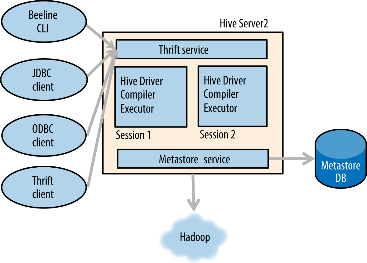
For more on Hive, see the Apache Hive site, or Programming Hive.

Example of Hive Code

Continuing the example of filter-join-filter, let’s see an implementation in Hive.

First, we will need to make tables for our data sets, shown in the following code. We will use external tables because that way if we were to delete the table, only the metadata (information about the name of table, column names, types, etc. in the metastore) will get deleted. The underlying data in HDFS still remains intact:

CREATE EXTERNAL TABLE foo(fooId BIGINT, fooVal INT, fooBarId BIGINT)
 ROW FORMAT DELIMITED
   FIELDS TERMINATED BY '|'
STORED AS TEXTFILE
LOCATION 'foo';

CREATE EXTERNAL TABLE bar(barId BIGINT, barVal INT)
 ROW FORMAT DELIMITED
   FIELDS TERMINATED BY '|'
STORED AS TEXTFILE
LOCATION 'bar';

You’ll notice this syntax is a little different from a typical RDBMS system, but any user familiar with SQL should be able to get the idea of what is going on. In short, we are making two tables named foo and bar. Their data is stored in text files with “|” as a column delimiter, and the files containing the data are located in the foo and bar directories, respectively, in HDFS.

Another thing to note is that we’re also defining the storage format in these statements. In this case we’re simply storing the data as delimited text files, but in a production application we’ll likely use an optimized binary format, such as Parquet, for storage. We’ll see a concrete example of this in not available. This is in contrast to most traditional data stores, such as an RDBMS, in which data is automatically converted into a proprietary, optimized format for that database.

Now, when that is done we can optionally (but it’s always recommended) run the command to compute statistics. This will allow Hive to select join strategies and execution plans better suited to the data based on its distribution. The commands for computing statistics in Hive for the preceding tables would look like:

ANALYZE TABLE foo COMPUTE STATISTICS;

ANALYZE TABLE bar COMPUTE STATISTICS;

The automatic population of Hive statistics is controlled by a property named hive.stats.autogather, which is set to true by default. However, the stats are only automatically computed if you are inserting data via a Hive insert statement, like INSERT OVERWRITE TABLE. If you are moving data into HDFS outside of Hive or using something like Flume to stream data into your Hive table’s HDFS location, you will have to run an ANALYZE TABLE TABLE NAME COMPUTE STATISTICS command explicitly to update the table statistics.

This will run map-only jobs that will read through the data and compute various statistics about it (min, max, etc.), which can then be used by the Hive query planner for queries on these tables later on.

When compute stats are done, we are ready to go. The following code shows how we would execute the filter-join-filter query in Hive:

SELECT
  *
FROM
  foo f JOIN bar b ON (f.fooBarId = b.barId)
WHERE
  f.fooVal < 500 AND
  f.fooVal + b.barVal < 1000;

As you’ll notice this is quite simple, especially for someone who is already familiar with SQL. There is no need to learn MapReduce, Pig, Crunch, Cascading, and so on.

A word of caution here is that Hive is not the best at optimization and sometimes, even to optimize, you may have to set a few configuration properties. For example, Hive supports various kinds of distributed joins: map join (also known as hash join), bucketed join, sorted bucketed merge join, and regular join. If your data sets meet certain prerequisites, some joins may lead to much better performance than others. However, older versions of Hive didn’t select the right join automatically, so the Hive compiler would rely on hints supplied by the query author to choose the right join for the query in question. Newer versions of Hive select the right join automatically, and as the project evolves more and more of these optimizations are being done automatically.

Also note that even though SQL is great for querying, it’s not the best language for expressing all forms of processing. For every processing problem that you are expressing in SQL, you should ask whether SQL is a good fit, or if you’re shoehorning the problem into it. Problems that use simple filtering and aggregation are a good fit for SQL. For example, if you need to find the user who was most active on Twitter in the past month, that is fairly easy to do in SQL (assuming you have access to the Twitter data set); you need to count Twitter activity for each user and then find the user with the highest count. On the other hand, machine learning, text processing, and graph algorithms are typically a poor fit for SQL. If you need to choose which advertisement to show to each Twitter user based on that user’s interests and friends, it is unlikely that SQL is the right tool.

Similar to Pig, Hive is an abstraction over MapReduce, unless you’re using one of the newer execution engines noted earlier. This means that Hive also hides all the MapReduce work behind the scenes. You should still make a habit of reviewing what Hive is doing under the hood to ensure it’s doing what you intend. You can do this by simply adding the word EXPLAIN before the query command. The next example shows what the explain plan looks like for our filter-join-filter query.

As you’ll see in the explain plan, the SQL query is mapped to three stages in Hive processing. Notice in the plan for stage 3 that in this example, Hive automatically figured out to do a map join (instead of the less performant regular join). Stage 3 populates a hash table equivalent to the query SELECT * FROM foo f WHERE f.fooVal < 500. This hash table is held in memory in all nodes of the cluster doing the join. Then, as shown in stage 4, the values from the bar table are simply read and joined against the in-memory hash table containing prefiltered values from the foo table:

EXPLAIN SELECT *
    > FROM foo f JOIN bar b ON (f.fooBarId = b.barId)
    > WHERE f.fooVal < 500 AND
    > f.fooVal + b.barVal < 1000
    > ;
OK
ABSTRACT SYNTAX TREE:


STAGE DEPENDENCIES:
  Stage-4 is a root stage
  Stage-3 depends on stages: Stage-4
  Stage-0 is a root stage

STAGE PLANS:
  Stage: Stage-4
    Map Reduce Local Work
      Alias -> Map Local Tables:
        f
          Fetch Operator
            limit: -1
      Alias -> Map Local Operator Tree:
        f
          TableScan
            alias: f
            Filter Operator
              predicate:
                  expr: (fooval < 500)
                  type: boolean
              HashTable Sink Operator
                condition expressions:
                  0 {fooid} {fooval} {foobarid}
                  1 {barid} {barval}
                handleSkewJoin: false
                keys:
                  0 [Column[foobarid]]
                  1 [Column[barid]]
                Position of Big Table: 1

  Stage: Stage-3
    Map Reduce
      Alias -> Map Operator Tree:
        b
          TableScan
            alias: b
            Map Join Operator
              condition map:
                   Inner Join 0 to 1
              condition expressions:
                0 {fooid} {fooval} {foobarid}
                1 {barid} {barval}
              handleSkewJoin: false
              keys:
                0 [Column[foobarid]]
                1 [Column[barid]]
              outputColumnNames: _col0, _col1, _col2, _col5, _col6
              Position of Big Table: 1
              Filter Operator
                predicate:
                    expr: ((_col1 < 500) and ((_col1 + _col6) < 1000))
                    type: boolean
                Select Operator
                  expressions:
                        expr: _col0
                        type: bigint
                        expr: _col1
                        type: int
                        expr: _col2
                        type: bigint
                        expr: _col5
                        type: bigint
                        expr: _col6
                        type: int
                  outputColumnNames: _col0, _col1, _col2, _col3, _col4
                  File Output Operator
                    compressed: false
                    GlobalTableId: 0
                    table:
                    input format: org.apache.hadoop.mapred.TextInputFormat
                    output format:\
                    org.apache.hadoop.hive.ql.io.HiveIgnoreKeyTextOutputFormat
                    serde: org.apache.hadoop.hive.serde2.lazy.LazySimpleSerDe
      Local Work:
        Map Reduce Local Work

  Stage: Stage-0
    Fetch Operator
      limit: -1

When to Use Hive

While this section mainly answers the question of when to use Hive for processing and querying data, it’s important to point out that one part of Hive, the Hive metastore, has become the de facto standard for storing metadata (table names, column names and types, etc.) in the Hadoop ecosystem, as explained in the section not available. Therefore, regardless of what engine you use, you will most likely always set up and use the Hive metastore to store metadata.

Hive of course is a good choice for queries that lend themselves to being expressed in SQL, particularly long-running queries where fault tolerance is desirable. Aside from queries, Hive can be a good choice if you’d like to write feature-rich, fault-tolerant, batch (i.e., not near-real-time) transformation or ETL jobs in a pluggable SQL engine. Let’s talk about these features in more detail:

SQL

Hive is a SQL engine for Hadoop. So is Impala and other engines not discussed here, like Apache Drill and Spark-SQL. So, if you care about writing your queries in SQL, you should probably only look at engines in this category.

Pluggable

Hive is arguably the most pluggable SQL engine in the ecosystem. Pluggability here can refer to several things. Hive supports writing custom data formats and writing code to serialize and deserialize (Hive SerDes) that data. Also, you can change the underlying execution engine in Hive from MapReduce to Tez to Spark (still pending at the time of writing). So, if switching between underlying general-purpose execution engines is important to you, Hive would be a good choice.

Batch

Hive is a batch engine. This means that you can’t expect results in real time. Certain other engines, like Impala, are, in general, faster than Hive. So, if speed is your primary motive, Hive may not be the best fit.

Fault-tolerant

Hive is fault-tolerant, whereas other engines, like Impala at the time of this writing, are not. That means if a node processing a part of the query fails while running, the entire query will fail in Impala, but in Hive the underlying task would be retried. If your queries are hours long, this is very likely undesirable, but if your queries are shorter a simple retry from the client should suffice. Therefore, if fault tolerance is very important to you, Hive is usually a good choice.

Feature-rich

So, if Hive is slow, why use it at all? Hive is the oldest SQL engine on Hadoop; therefore, at the time of this writing, it has more features, in general, than newer engines. For example, at the time of this writing, Impala doesn’t support nested data types (structs, arrays, maps, etc.). If representing data natively in those nested types is important to you, Hive is likely a very good choice.

Impala Overview

Impala has a shared nothing architecture, which allows for system-level fault tolerance and huge scalability that allows Impala to remain performant as the number of users and concurrent queries increases.

Impala’s architecture includes the Impala daemons (impalad), the catalog service, and the statestore. Impala daemons run on every node in the cluster, and each daemon is capable of acting as the query planner, the query coordinator, and a query execution engine. To connect to Impala, the client uses JDBC, ODBC, impala-shell, or connects directly via Apache Thrift to connect to one of the Impala daemons. All Impala daemons are identical and interchangeable, so the client will typically connect to a load balancer that will direct the connection to an active daemon. The daemon the client connects to will act as a query planner and coordinator for this query.

The query planner is responsible for parsing out the given SQL query and producing an execution plan. The query coordinator takes the plan and then assigns parts of it to the rest of the Impala daemons to execute. The Impala architecture is illustrated in Figure 1-11.

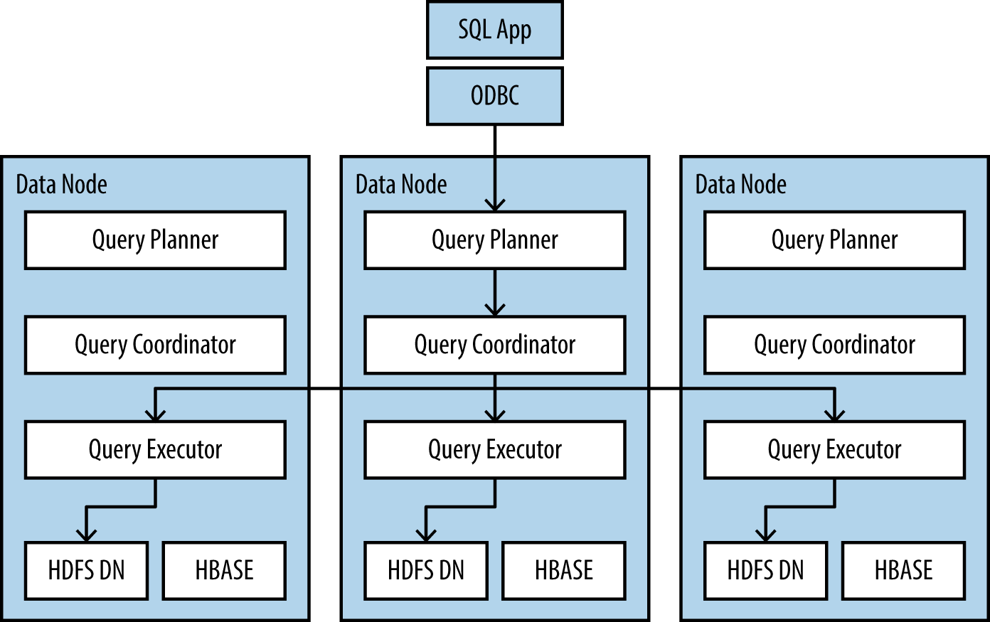
Note that unlike other database management systems such as an RDBMS, Impala does not have to implement the underlying data store, because this is off-loaded to HDFS and HBase. Impala also doesn’t have to implement the table and database management solution since this is implemented by the Hive metastore. This allows Impala to focus on its core functionality, which is executing queries as fast as possible.

Because Impala aims to be a distributed MPP database on top of Hadoop, the intent is to implement various distributed join strategies commonly found in such MPP databases. At the time of this writing, two such join strategies have been implemented: broadcast hash joins and partitioned hash joins. If you’d like to review the internals of such join strategies and how they are implemented in Impala, please see not available.

Speed-Oriented Design

There are several design decisions that reduce Impala’s query latency compared to other SQL-in-Hadoop solutions.

Impala Example

Although the inner workings of Impala can seem quite complex, using Impala is actually fairly easy. You can start impala-shell, the Impala command-line interface, and begin submitting queries like so:

CONNECT <impalaDaemon host name or loadbalancer>;

-- Make sure Impala has the latest metadata about which tables exist, etc.
-- from the Hive metastore
INVALIDATE METADATA;

SELECT
  *
FROM
  foo f JOIN bar b ON (f.fooBarId = b.barId)
WHERE
  f.fooVal < 500 AND
  f.fooVal + b.barVal < 1000;

This code connects to Impala, updates the metadata from Hive, and runs our query. You can immediately see why most developers prefer the SQL version of this code to the MapReduce version we saw earlier in the chapter.

To see the execution plan of a query in Impala, you simply add the word EXPLAIN before your query. The syntax is identical to that of Hive, but the resulting query plan is completely different. Because Impala is implemented as an MPP data warehouse, the execution plans use similar operators and look similar to those of Oracle and Netezza. These are very different from the MapReduce-based plans that are produced by Hive.

Here is the explain plan of the query just shown:

+------------------------------------------------------------------------------+
| Explain String                                                               |
+------------------------------------------------------------------------------+
| Estimated Per-Host Requirements: Memory=32.00MB VCores=2                     |
| WARNING: The following tables are missing relevant table                     |
|  and/or column statistics.                                                   |
| default.bar, default.foo                                                     |
|                                                                              |
| 04:EXCHANGE [PARTITION=UNPARTITIONED]                                        |
| |                                                                            |
| 02:HASH JOIN [INNER JOIN, BROADCAST]                                         |
| |  hash predicates: f.fooBarId = b.barId                                     |
| |  other predicates: f.fooVal + b.barVal < 1000                              |
| |                                                                            |
| |--03:EXCHANGE [BROADCAST]                                                   |
| |  |                                                                         |
| |  01:SCAN HDFS [default.bar b]                                              |
| |     partitions=1/1 size=7.61KB                                             |
| |                                                                            |
| 00:SCAN HDFS [default.foo f]                                                 |
|    partitions=1/1 size=1.04KB                                                |
|    predicates: f.fooVal < 500                                                |
+------------------------------------------------------------------------------+

We can see that Impala first scans table foo and filters it with the predicate in the query. The plan shows the filtering predicate and the table size after the filtering as estimated by the Impala optimizer. The results of the filter operation are joined with table bar via a broadcast join, and the plan also shows the join columns and the additional filter.

Impala also has a web UI, by default on port 25000 on each Impala daemon. This web UI gives access to query profiles. Query profiles look similar to execution plans, but they are created after the query is executed—so in addition to the estimated size, a query profile also contains additional runtime information such as the rates at which tables were scanned, the actual data sizes, the amount of memory used, the execution times, and so on. This information is very useful for improving query performance.

When to Use Impala

As we’ve discussed, there are a few options for running SQL on data in Hadoop, Hive being the most popular of them. So when to use Hive versus Impala?

We think the answer to that question depends on your use case, but more interesting is that it will change with time as both Hive and Impala evolve. As of this writing, even though Impala is much faster than Hive on MapReduce and is highly concurrent, it is not fault-tolerant like Hive, nor does it have all the features that Hive has (like complex data types—maps, structs, arrays, etc.). Therefore, our recommendation is to use Impala where possible to make use of the higher speed. In particular, if your organization has hundreds of users who will need to run SQL queries on Hadoop concurrently, Impala is known to scale very well to fit such a requirement. However, let’s say your query needs to scan so much data (e.g., hundreds of terabytes) that even with Impala’s performance the query will take hours due to the sheer amount of I/O needed. In that scenario, the ability to recover the query from a node failure without restarting is critical. Hive offers this functionality and would be our recommendation in such a case. Also worth pointing out is the fact that at the time of this writing, Impala lacks certain features that exist in Hive. The most important one is the ability to process nested data types (that’s currently under development in Impala). Therefore, if using nested data types is critical to your application, we recommend you use Hive. As Hive and Impala evolve, this gap is expected to change.

Another important decision factor is the support for custom file formats. Hive supports all the popular file formats in the ecosystem (e.g., delimited text, Parquet, Avro, RCFile, SequenceFile) as well as custom file formats (e.g., JSON) by means of writing a pluggable SerDe (serializer/deserializer). However, Impala only supports the same popular Hadoop file formats; it doesn’t provide support for writing custom file formats. In such cases, you can use Hive to read data directly in the format in question, or convert the data in Hive to a popular file format in the Hadoop ecosystem and then use Impala to query that data set.

Also note that while the choice between Impala and Hive may seem complicated now, it’s relatively simple to switch between the two since they share the same metadata. For example, a table created and populated via Hive is readable via Impala and vice versa without any additional steps required to transfer between the two systems.