Analysis of Financial Time Series, Third Edition

3.14 Application

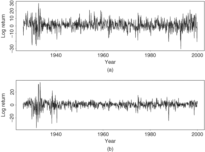
In this section, we apply the volatility models discussed in this chapter to investigate some problems of practical importance. The data used are the monthly log returns of IBM stock and the S&P 500 index from January 1926 to December 1999. There are 888 observations, and the returns are in percentages and include dividends. Figure 3.11 shows the time plots of the two return series. Note that the result of this section was obtained by the RATS program.

Figure 3.11 Time plots of monthly log returns for (a) IBM stock and (b) S&P 500 index. Sample period is from January 1926 to December 1999. Returns are in percentages and include dividends.

Example 3.4

The questions we address here are whether the daily volatility of a stock is lower in the summer and, if so, by how much. Affirmative answers to these two questions have practical implications in stock option pricing. We use the monthly log returns of IBM stock shown in Figure 3.11(a) as an illustrative example.

Denote the monthly log return series by rt. If Gaussian GARCH models are entertained, we obtain the GARCH(1,1) model:

3.42

for the series. The standard errors of the two parameters in the mean equation are 0.222 and 0.037, respectively, whereas those of the parameters in the volatility equation are 0.947, ...