Automation for Robotics

Introduction

I.1. State representation

Biological, economic and other mechanical systems surrounding us can often be described by a differential equation such as:

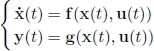
under the hypothesis that the time t in which the system evolves is continuous [JAU 05]. The vector u(t) is the input (or control) of the system. Its value may be chosen arbitrarily for all t. The vector y(t) is the output of the system and can be measured with a certain degree of accuracy. The vector x(t) is called the state of the system. It represents the memory of the system, in other words the information needed by the system in order to predict its own future, for a known input u(t). The first of the two equations is called the evolution equation. It is a differential equation that enables us to know where the state (t) is headed knowing its value at the present moment t and the control u(t) that we are currently exerting. The second equation is called the observation equation. It allows us to calculate the output vector y(t), knowing the state and control at time t. Note, however, that, unlike the evolution equation, this equation is not a differential equation as it does not involve the derivatives of the signals. The two equations given above form the state representation of the system.

It is sometimes useful to consider a discrete time k, with   where  is the set of integers. If, for instance, the universe is being ...