Bayesian Estimation and Tracking: A Practical Guide

13.1 Analytical Kalman Filters

There are many dynamic systems where either the dynamic or observation equation is linear. This is true for most of the case studies considered in this book.

For some cases, the dynamic equation is linear while the observation equation is highly nonlinear. For these, the linear Kalman filter prediction Equations (6.3) and (6.6) can always be used for the state and state covariance predictions in lieu of any of the other prediction methods. For other tracking problems, the dynamic equation may be nonlinear while the observation equation is linear. For these problems, the reverse is true: one must use one of the nonlinear methods for state prediction, but the linear Kalman filter predictions (6.9)–(6.12) can be used for observation prediction. Finally, if both the dynamic and observation equations are linear, all of the LKF prediction equations are used.

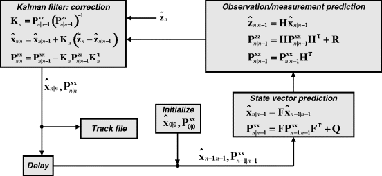
A process diagram for the LKF is presented in Figure 13.1

Figure 13.1 Graphical presentation of the linear Kalman filter process flow.

When the dynamic and/or observation equation is nonlinear, one of the nonlinear methods developed in Chapters 7–12 must be used. The method that has seen the most use over the past 50 years is the EKF. As we have shown in Chapter 7, the EKF involves an expansion of the nonlinear functions in a first-order Taylor polynomial resulting in a Kalman filter with the same form ...