Binary Digital Image Processing

142 BINARY DIGITAL IMAGE PROCESSING

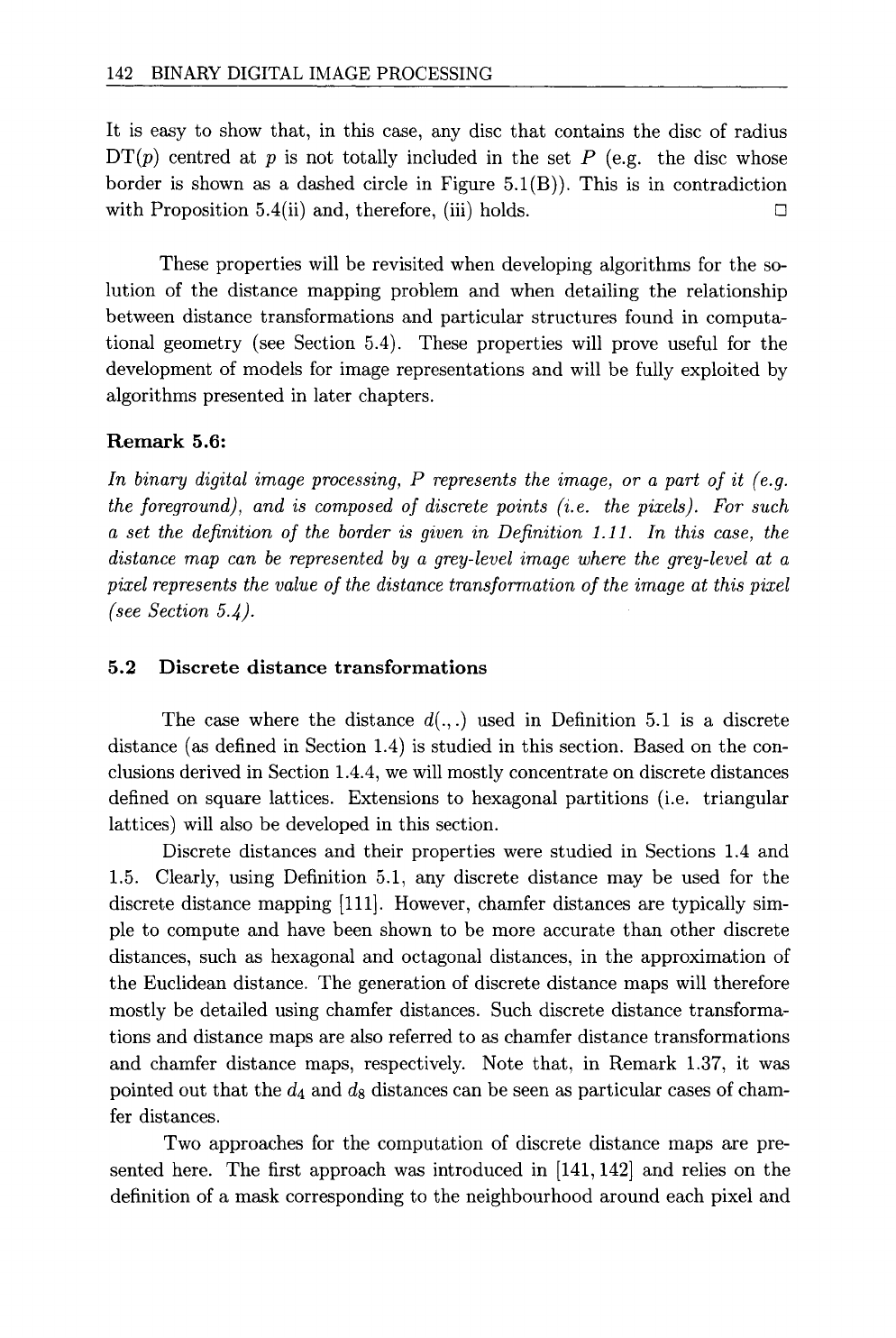
It is easy to show that, in this case, any disc that contains the disc of radius

DT(p) centred at p is not totally included in the set P (e.g. the disc whose

border is shown as a dashed circle in Figure 5.1(B)). This is in contradiction

with Proposition 5.4(ii) and, therefore, (iii) holds. [::]

These properties will be revisited when developing algorithms for the so-

lution of the distance mapping problem and when detailing the relationship

between distance transformations and particular structures found in computa-

tional geometry (see Section 5.4). These properties will prove useful for the

development of models for image representations and will be fully exploited by

algorithms presented in later chapters.

Remark 5.6:

In binary digital image processing, P represents the image, or a part of it (e.g.

the foreground), and is composed of discrete points (i.e. the pixels). For such

a set the definition of the border is given in Definition 1.11. In this case, the

distance map can be represented by a grey-level image where the grey-level at a

pixel represents the value of the distance transformation of the image at this pixel

(see Section 5.~).

5.2 Discrete distance transformations

The case where the distance d(.,.) used in Definition 5.1 is a discrete

distance (as defined in Section 1.4) is studied in this section. Based on the con-

clusions derived in Section 1.4.4, we will mostly concentrate on discrete distances

defined on square lattices. Extensions to hexagonal partitions (i.e. triangular

lattices) will also be developed in this section.

Discrete distances and their properties were studied in Sections 1.4 and

1.5. Clearly, using Definition 5.1, any discrete distance may be used for the

discrete distance mapping [111]. However, chamfer distances are typically sim-

ple to compute and have been shown to be more accurate than other discrete

distances, such as hexagonal and octagonal distances, in the approximation of

the Euclidean distance. The generation of discrete distance maps will therefore

mostly be detailed using chamfer distances. Such discrete distance transforma-

tions and distance maps are also referred to as chamfer distance transformations

and chamfer distance maps, respectively. Note that, in Remark 1.37, it was

pointed out that the d4 and d8 distances can be seen as particular cases of cham-

fer distances.

Two approaches for the computation of discrete distance maps are pre-

sented here. The first approach was introduced in [141,142] and relies on the

definition of a mask corresponding to the neighbourhood around each pixel and