Chapter 4. The Cassandra Query Language
In this chapter, you’ll gain an understanding of Cassandra’s data model and how that data model is implemented by the Cassandra Query Language (CQL). We’ll show how CQL supports Cassandra’s design goals and look at some general behavior characteristics.
For developers and administrators coming from the relational world, the Cassandra data model can be difficult to understand initially. Some terms, such as “keyspace,” are completely new, and some, such as “column,” exist in both worlds but have slightly different meanings. The syntax of CQL is similar in many ways to SQL, but with some important differences. For those familiar with NoSQL technologies such as Dynamo or Bigtable, it can also be confusing, because although Cassandra may be based on those technologies, its own data model is significantly different.
So in this chapter, we start from relational database terminology and introduce Cassandra’s view of the world. Along the way we’ll get more familiar with CQL and learn how it implements this data model.
The Relational Data Model
In a relational database, we have the database itself, which is the outermost container that might correspond to a single application. The database contains tables. Tables have names and contain one or more columns, which also have names. When we add data to a table, we specify a value for every column defined; if we don’t have a value for a particular column, we use null. This new entry adds a row to the table, which we can later read if we know the row’s unique identifier (primary key), or by using a SQL statement that expresses some criteria that row might meet. If we want to update values in the table, we can update all of the rows or just some of them, depending on the filter we use in a “where” clause of our SQL statement.
Now that we’ve had this review, we’re in good shape to look at Cassandra’s data model in terms of its similarities and differences.
Cassandra’s Data Model
In this section, we’ll take a bottom-up approach to understanding Cassandra’s data model.
The simplest data store you would conceivably want to work with might be an array or list. It would look like Figure 4-1.

Figure 4-1. A list of values
If you persisted this list, you could query it later, but you would have to either examine each value in order to know what it represented, or always store each value in the same place in the list and then externally maintain documentation about which cell in the array holds which values. That would mean you might have to supply empty placeholder values (nulls) in order to keep the predetermined size of the array in case you didn’t have a value for an optional attribute (such as a fax number or apartment number). An array is a clearly useful data structure, but not semantically rich.
So we’d like to add a second dimension to this list: names to match the values. We’ll give names to each cell, and now we have a map structure, as shown in Figure 4-2.
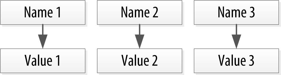
Figure 4-2. A map of name/value pairs
This is an improvement because we can know the names of our values. So if we decided that our map would hold User information, we could have column names like first_name, last_name, phone, email, and so on. This is a somewhat richer structure to work with.
But the structure we’ve built so far works only if we have one instance of a given entity, such as a single person, user, hotel, or tweet. It doesn’t give us much if we want to store multiple entities with the same structure, which is certainly what we want to do. There’s nothing to unify some collection of name/value pairs, and no way to repeat the same column names. So we need something that will group some of the column values together in a distinctly addressable group. We need a key to reference a group of columns that should be treated together as a set. We need rows. Then, if we get a single row, we can get all of the name/value pairs for a single entity at once, or just get the values for the names we’re interested in. We could call these name/value pairs columns. We could call each separate entity that holds some set of columns rows. And the unique identifier for each row could be called a row key or primary key. Figure 4-3 shows the contents of a simple row: a primary key, which is itself one or more columns, and additional columns.
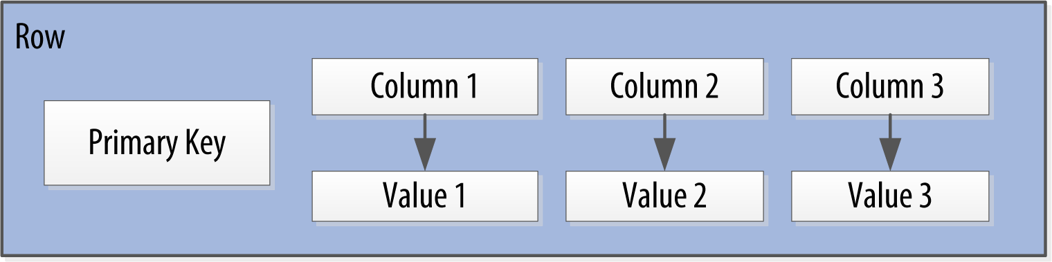
Figure 4-3. A Cassandra row
Cassandra defines a table to be a logical division that associates similar data. For example, we might have a user table, a hotel table, an address book table, and so on. In this way, a Cassandra table is analogous to a table in the relational world.
Now we don’t need to store a value for every column every time we store a new entity. Maybe we don’t know the values for every column for a given entity. For example, some people have a second phone number and some don’t, and in an online form backed by Cassandra, there may be some fields that are optional and some that are required. That’s OK. Instead of storing null for those values we don’t know, which would waste space, we just won’t store that column at all for that row. So now we have a sparse, multidimensional array structure that looks like Figure 4-4.
When designing a table in a traditional relational database, you’re typically dealing with “entities,” or the set of attributes that describe a particular noun (hotel, user, product, etc.). Not much thought is given to the size of the rows themselves, because row size isn’t negotiable once you’ve decided what noun your table represents. However, when you’re working with Cassandra, you actually have a decision to make about the size of your rows: they can be wide or skinny, depending on the number of columns the row contains.
A wide row means a row that has lots and lots (perhaps tens of thousands or even millions) of columns. Typically there is a smaller number of rows that go along with so many columns. Conversely, you could have something closer to a relational model, where you define a smaller number of columns and use many different rows—that’s the skinny model. We’ve already seen a skinny model in Figure 4-4.
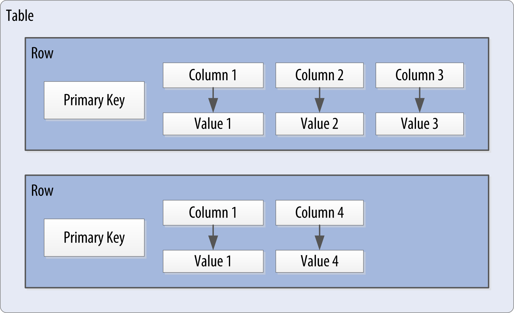
Figure 4-4. A Cassandra table
Cassandra uses a special primary key called a composite key (or compound key) to represent wide rows, also called partitions. The composite key consists of a partition key, plus an optional set of clustering columns. The partition key is used to determine the nodes on which rows are stored and can itself consist of multiple columns. The clustering columns are used to control how data is sorted for storage within a partition. Cassandra also supports an additional construct called a static column, which is for storing data that is not part of the primary key but is shared by every row in a partition.
Figure 4-5 shows how each partition is uniquely identified by a partition key, and how the clustering keys are used to uniquely identify the rows within a partition.
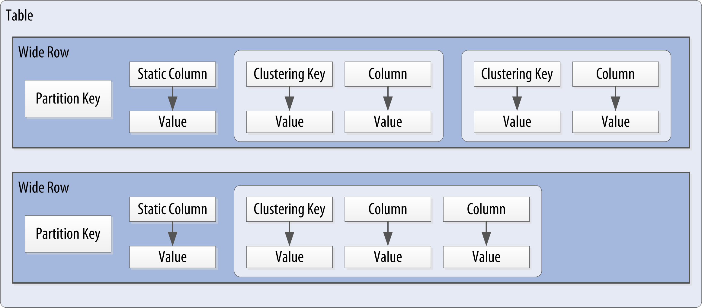
Figure 4-5. A Cassandra wide row
For this chapter, we will concern ourselves with simple primary keys consisting of a single column. In these cases, the primary key and the partition key are the same, because we have no clustering columns. We’ll examine more complex primary keys in Chapter 5.
Putting this all together, we have the basic Cassandra data structures:
- The column, which is a name/value pair
- The row, which is a container for columns referenced by a primary key
- The table, which is a container for rows
- The keyspace, which is a container for tables
- The cluster, which is a container for keyspaces that spans one or more nodes
So that’s the bottom-up approach to looking at Cassandra’s data model. Now that we know the basic terminology, let’s examine each structure in more detail.
Clusters
As previously mentioned, the Cassandra database is specifically designed to be distributed over several machines operating together that appear as a single instance to the end user. So the outermost structure in Cassandra is the cluster, sometimes called the ring, because Cassandra assigns data to nodes in the cluster by arranging them in a ring.
Keyspaces
A cluster is a container for keyspaces. A keyspace is the outermost container for data in Cassandra, corresponding closely to a relational database. In the same way that a database is a container for tables in the relational model, a keyspace is a container for tables in the Cassandra data model. Like a relational database, a keyspace has a name and a set of attributes that define keyspace-wide behavior.
Because we’re currently focusing on the data model, we’ll leave questions about setting up and configuring clusters and keyspaces until later. We’ll examine these topics in Chapter 7.
Tables
A table is a container for an ordered collection of rows, each of which is itself an ordered collection of columns. The ordering is determined by the columns, which are identified as keys. We’ll soon see how Cassandra uses additional keys beyond the primary key.
When you write data to a table in Cassandra, you specify values for one or more columns. That collection of values is called a row. At least one of the values you specify must be a primary key that serves as the unique identifier for that row.
Let’s go back to the user table we created in the previous chapter. Remember how we wrote a row of data and then read it using the SELECT command in cqlsh:
cqlsh:my_keyspace> SELECT * FROM user WHERE first_name='Bill';

 first_name | last_name
------------+-----------
       Bill |    Nguyen

(1 rows)
You’ll notice in the last row that the shell tells us that one row was returned. It turns out to be the row identified by the first_name “Bill”. This is the primary key that identifies this row.
Data Access Requires a Primary Key
This is an important detail—the SELECT, INSERT, UPDATE, and DELETE commands in CQL all operate in terms of rows.
As we stated earlier, we don’t need to include a value for every column when we add a new row to the table. Let’s test this out with our user table using the ALTER TABLE command and then view the results using the DESCRIBE TABLE command:
cqlsh:my_keyspace> ALTER TABLE user ADD title text;
cqlsh:my_keyspace> DESCRIBE TABLE user;

CREATE TABLE my_keyspace.user (
    first_name text PRIMARY KEY,
    last_name text,
    title text
) ...
We see that the title column has been added. Note that we’ve shortened the output to omit the various table settings. You’ll learn more about these settings and how to configure them in Chapter 7.
Now, let’s write a couple of rows, populate different columns for each, and view the results:
cqlsh:my_keyspace> INSERT INTO user (first_name, last_name, title)
  VALUES ('Bill', 'Nguyen', 'Mr.');
cqlsh:my_keyspace> INSERT INTO user (first_name, last_name) VALUES
  ('Mary', 'Rodriguez');
cqlsh:my_keyspace> SELECT * FROM user;

 first_name | last_name | title
------------+-----------+-------
       Mary | Rodriguez |  null
       Bill |    Nguyen |   Mr.

(2 rows)
Now that we’ve learned more about the structure of a table and done some data modeling, let’s dive deeper into columns.
Columns
A column is the most basic unit of data structure in the Cassandra data model. So far we’ve seen that a column contains a name and a value. We constrain each of the values to be of a particular type when we define the column. We’ll want to dig into the various types that are available for each column, but first let’s take a look into some other attributes of a column that we haven’t discussed yet: timestamps and time to live. These attributes are key to understanding how Cassandra uses time to keep data current.
Timestamps
Each time you write data into Cassandra, a timestamp is generated for each column value that is updated. Internally, Cassandra uses these timestamps for resolving any conflicting changes that are made to the same value. Generally, the last timestamp wins.
Let’s view the timestamps that were generated for our previous writes by adding the writetime() function to our SELECT command. We’ll do this on the lastname column and include a couple of other values for context:
cqlsh:my_keyspace> SELECT first_name, last_name,
  writetime(last_name) FROM user;

 first_name | last_name | writetime(last_name)
------------+-----------+----------------------
       Mary | Rodriguez |     1434591198790252
       Bill |    Nguyen |     1434591198798235

(2 rows)
We might expect that if we ask for the timestamp on first_name we’d get a similar result. However, it turns out we’re not allowed to ask for the timestamp on primary key columns:
cqlsh:my_keyspace> SELECT WRITETIME(first_name) FROM user;
InvalidRequest: code=2200 [Invalid query] message="Cannot use
  selection function writeTime on PRIMARY KEY part first_name"
Cassandra also allows us to specify a timestamp we want to use when performing writes. To do this, we’ll use the CQL UPDATE command for the first time. We’ll use the optional USING TIMESTAMP option to manually set a timestamp (note that the timestamp must be later than the one from our SELECT command, or the UPDATE will be ignored):
cqlsh:my_keyspace> UPDATE user USING TIMESTAMP 1434373756626000
  SET last_name = 'Boateng' WHERE first_name = 'Mary' ;
cqlsh:my_keyspace> SELECT first_name, last_name,
  WRITETIME(last_name) FROM user WHERE first_name = 'Mary';

 first_name | last_name   | writetime(last_name)
------------+-------------+---------------------
  Mary      | Boateng     | 1434373756626000

(1 rows)
This statement has the effect of adding the last name column to the row identified by the primary key “Mary”, and setting the timestamp to the value we provided.
Working with Timestamps
Setting the timestamp is not required for writes. This functionality is typically used for writes in which there is a concern that some of the writes may cause fresh data to be overwritten with stale data. This is advanced behavior and should be used with caution.
There is currently not a way to convert timestamps produced by writetime() into a more friendly format in cqlsh.
Time to live (TTL)
One very powerful feature that Cassandra provides is the ability to expire data that is no longer needed. This expiration is very flexible and works at the level of individual column values. The time to live (or TTL) is a value that Cassandra stores for each column value to indicate how long to keep the value.
The TTL value defaults to null, meaning that data that is written will not expire. Let’s show this by adding the TTL() function to a SELECT command in cqlsh to see the TTL value for Mary’s last name:
cqlsh:my_keyspace> SELECT first_name, last_name, TTL(last_name)
  FROM user WHERE first_name = 'Mary';

 first_name | last_name | ttl(last_name)
------------+-----------+----------------
       Mary |   Boateng |           null

(1 rows)
Now let’s set the TTL on the last name column to an hour (3,600 seconds) by adding the USING TTL option to our UPDATE command:
cqlsh:my_keyspace> UPDATE user USING TTL 3600 SET last_name =
  'McDonald' WHERE first_name = 'Mary' ;
cqlsh:my_keyspace> SELECT first_name, last_name, TTL(last_name)
  FROM user WHERE first_name = 'Mary';

 first_name | last_name   | ttl(last_name)
------------+-------------+---------------
  Mary      |  McDonald   |           3588

(1 rows)
As you can see, the clock is already counting down our TTL, reflecting the several seconds it took to type the second command. If we run this command again in an hour, Mary’s last_name will be set to null. We can also set TTL on INSERTS using the same USING TTL option.
Using TTL
Remember that TTL is stored on a per-column level. There is currently no mechanism for setting TTL at a row level directly. As with the timestamp, there is no way to obtain or set the TTL value of a primary key column, and the TTL can only be set for a column when we provide a value for the column.
If we want to set TTL across an entire row, we must provide a value for every non-primary key column in our INSERT or UPDATE command.
CQL Types
Now that we’ve taken a deeper dive into how Cassandra represents columns including time-based metadata, let’s look at the various types that are available to us for our values.
As we’ve seen in our exploration so far, each column in our table is of a specified type. Up until this point, we’ve only used the varchar type, but there are plenty of other options available to us in CQL, so let’s explore them.
CQL supports a flexible set of data types, including simple character and numeric types, collections, and user-defined types. We’ll describe these data types and provide some examples of how they might be used to help you learn to make the right choice for your data model.
Numeric Data Types
CQL supports the numeric types you’d expect, including integer and floating-point numbers. These types are similar to standard types in Java and other languages:
int- A 32-bit signed integer (as in Java)
bigint- A 64-bit signed long integer (equivalent to a Java
long) smallint- A 16-bit signed integer (equivalent to a Java
short) tinyint- An 8-bit signed integer (as in Java)
varint- A variable precision signed integer (equivalent to
java.math.BigInteger) float- A 32-bit IEEE-754 floating point (as in Java)
double- A 64-bit IEEE-754 floating point (as in Java)
decimal- A variable precision decimal (equivalent to
java.math.BigDecimal)
Additional Integer Types
The smallint and tinyint types were added in the Cassandra 2.2 release.
While enumerated types are common in many languages, there is no direct equivalent in CQL. A common practice is to store enumerated values as strings. For example, using the Enum.name() method to convert an enumerated value to a String for writing to Cassandra as text, and the Enum.valueOf() method to convert from text back to the enumerated value.
Textual Data Types
CQL provides two data types for representing text, one of which we’ve made quite a bit of use of already (text):
text,varchar- Synonyms for a UTF-8 character string
ascii- An ASCII character string
UTF-8 is the more recent and widely used text standard and supports internationalization, so we recommend using text over ascii when building tables for new data. The ascii type is most useful if you are dealing with legacy data that is in ASCII format.
Setting the Locale in cqlsh
By default, cqlsh prints out control and other unprintable characters using a backslash escape. You can control how cqlsh displays non-ASCII characters by setting the locale via the $LANG environment variable before running the tool. See the cqlsh command HELP TEXT_OUTPUT for more information.
Time and Identity Data Types
The identity of data elements such as rows and partitions is important in any data model in order to be able to access the data. Cassandra provides several types which prove quite useful in defining unique partition keys. Let’s take some time (pun intended) to dig into these:
timestamp-
While we noted earlier that each column has a timestamp indicating when it was last modified, you can also use a timestamp as the value of a column itself. The time can be encoded as a 64-bit signed integer, but it is typically much more useful to input a timestamp using one of several supported ISO 8601 date formats. For example:
2015-06-15 20:05-0700
2015-06-15 20:05:07-0700
2015-06-15 20:05:07.013-0700
2015-06-15T20:05-0700
2015-06-15T20:05:07-0700
2015-06-15T20:05:07.013+-0700
The best practice is to always provide time zones rather than relying on the operating system time zone configuration.
date,time-
Releases through Cassandra 2.1 only had the
timestamptype to represent times, which included both a date and a time of day. The 2.2 release introduceddateandtimetypes that allowed these to be represented independently; that is, a date without a time, and a time of day without reference to a specific date. As withtimestamp, these types support ISO 8601 formats.Although there are new
java.timetypes available in Java 8, thedatetype maps to a custom type in Cassandra in order to preserve compatibility with older JDKs. Thetimetype maps to a Javalongrepresenting the number of nanoseconds since midnight. uuid-
A universally unique identifier (UUID) is a 128-bit value in which the bits conform to one of several types, of which the most commonly used are known as Type 1 and Type 4. The CQL
uuidtype is a Type 4 UUID, which is based entirely on random numbers. UUIDs are typically represented as dash-separated sequences of hex digits. For example:1a6300ca-0572-4736-a393-c0b7229e193e
The
uuidtype is often used as a surrogate key, either by itself or in combination with other values.Because UUIDs are of a finite length, they are not absolutely guaranteed to be unique. However, most operating systems and programming languages provide utilities to generate IDs that provide adequate uniqueness, and
cqlshdoes as well. You can obtain a Type 4 UUID value via theuuid()function and use this value in anINSERTorUPDATE. timeuuid-
This is a Type 1 UUID, which is based on the MAC address of the computer, the system time, and a sequence number used to prevent duplicates. This type is frequently used as a conflict-free timestamp.
cqlshprovides several convenience functions for interacting with thetimeuuidtype:now(),dateOf()andunixTimestampOf().The availability of these convenience functions is one reason why
timeuuidtends to be used more frequently thanuuid.
Building on our previous examples, we might determine that we’d like to assign a unique ID to each user, as first_name is perhaps not a sufficiently unique key for our user table. After all, it’s very likely that we’ll run into users with the same first name at some point. If we were starting from scratch, we might have chosen to make this identifier our primary key, but for now we’ll add it as another column.
Primary Keys Are Forever
After you create a table, there is no way to modify the primary key, because this controls how data is distributed within the cluster, and even more importantly, how it is stored on disk.
Let’s add the identifier using a uuid :
cqlsh:my_keyspace> ALTER TABLE user ADD id uuid;
Next, we’ll insert an ID for Mary using the uuid() function and then view the results:
cqlsh:my_keyspace> UPDATE user SET id = uuid() WHERE first_name =
  'Mary';
cqlsh:my_keyspace> SELECT first_name, id FROM user WHERE
  first_name = 'Mary';

 first_name | id
------------+--------------------------------------
       Mary | e43abc5d-6650-4d13-867a-70cbad7feda9

(1 rows)
Notice that the id is in UUID format.
Now we have a more robust table design, which we can extend with even more columns as we learn about more types.
Other Simple Data Types
CQL provides several other simple data types that don’t fall nicely into one of the categories we’ve looked at already:
boolean-
This is a simple true/false value. The
cqlshis case insensitive in accepting these values but outputsTrueorFalse. blob-
A binary large object (blob) is a colloquial computing term for an arbitrary array of bytes. The CQL blob type is useful for storing media or other binary file types. Cassandra does not validate or examine the bytes in a blob. CQL represents the data as hexadecimal digits—for example,
0x00000ab83cf0. If you want to encode arbitrary textual data into the blob you can use thetextAsBlob()function in order to specify values for entry. See thecqlshhelp functionHELP BLOB_INPUTfor more information. inet-
This type represents IPv4 or IPv6 Internet addresses.
cqlshaccepts any legal format for defining IPv4 addresses, including dotted or non-dotted representations containing decimal, octal, or hexadecimal values. However, the values are represented using the dotted decimal format incqlshoutput—for example,192.0.2.235.IPv6 addresses are represented as eight groups of four hexadecimal digits, separated by colons—for example,
2001:0db8:85a3:0000:0000:8a2e:0370:7334. The IPv6 specification allows the collapsing of consecutive zero hex values, so the preceding value is rendered as follows when read usingSELECT:2001:db8:85a3:a::8a2e:370:7334. counter-
The counter data type provides 64-bit signed integer, whose value cannot be set directly, but only incremented or decremented. Cassandra is one of the few databases that provides race-free increments across data centers. Counters are frequently used for tracking statistics such as numbers of page views, tweets, log messages, and so on. The
countertype has some special restrictions. It cannot be used as part of a primary key. If a counter is used, all of the columns other than primary key columns must be counters. -
A Warning About Counters
Remember: the increment and decrement operators are not idempotent. There is no operation to reset a counter directly, but you can approximate a reset by reading the counter value and decrementing by that value. Unfortunately, this is not guaranteed to work perfectly, as the counter may have been changed elsewhere in between reading and writing.
Collections
Let’s say we wanted to extend our user table to support multiple email addresses. One way to do this would be to create additional columns such as email2, email3, and so on. While this is an approach that will work, it does not scale very well and might cause a lot of rework. It is much simpler to deal with the email addresses as a group or “collection.” CQL provides three collection types to help us out with these situations: sets, lists, and maps. Let’s now take a look at each of them:
set-
The
setdata type stores a collection of elements. The elements are unordered, butcqlshreturns the elements in sorted order. For example, text values are returned in alphabetical order. Sets can contain the simple types we reviewed earlier as well as user-defined types (which we’ll discuss momentarily) and even other collections. One advantage of usingsetis the ability to insert additional items without having to read the contents first.Let’s modify our
usertable to add a set of email addresses:cqlsh:my_keyspace> ALTER TABLE user ADD emails set<text>;
Then we’ll add an email address for Mary and check that it was added successfully:
cqlsh:my_keyspace> UPDATE user SET emails = {
  'mary@example.com' } WHERE first_name = 'Mary';
cqlsh:my_keyspace> SELECT emails FROM user WHERE first_name =
  'Mary';

 emails
----------------------
 {'mary@example.com'}

(1 rows)
Note that in adding that first email address, we replaced the previous contents of the set, which in this case was
null. We can add another email address later without replacing the whole set by using concatenation:cqlsh:my_keyspace> UPDATE user SET emails = emails + { 'mary.mcdonald.AZ@gmail.com' } WHERE first_name = 'Mary'; cqlsh:my_keyspace> SELECT emails FROM user WHERE first_name = 'Mary'; emails --------------------------------------------------- {'mary.mcdonald.AZ@gmail.com', 'mary@example.com'} (1 rows) list-
The
listdata type contains an ordered list of elements. By default, the values are stored in order of insertion. Let’s modify ourusertable to add a list of phone numbers:cqlsh:my_keyspace> ALTER TABLE user ADD phone_numbers list<text>;
Then we’ll add a phone number for Mary and check that it was added successfully:
cqlsh:my_keyspace> UPDATE user SET phone_numbers = [
  '1-800-999-9999' ] WHERE first_name = 'Mary';
cqlsh:my_keyspace> SELECT phone_numbers FROM user WHERE
  first_name = 'Mary';

 phone_numbers
--------------------
 ['1-800-999-9999']

(1 rows)
Let’s add a second number by appending it:
cqlsh:my_keyspace> UPDATE user SET phone_numbers =
  phone_numbers + [ '480-111-1111' ] WHERE first_name = 'Mary';
cqlsh:my_keyspace> SELECT phone_numbers FROM user WHERE
  first_name = 'Mary';

 phone_numbers
------------------------------------
 ['1-800-999-9999', '480-111-1111']

(1 rows)
The second number we added now appears at the end of the list.
Note
We could also have prepended the number to the front of the list by reversing the order of our values:
SET phone_numbers = [‘4801234567’] + phone_numbers.We can replace an individual item in the list when we reference it by its index:
cqlsh:my_keyspace> UPDATE user SET phone_numbers[1] =
  '480-111-1111' WHERE first_name = 'Mary';
As with sets, we can also use the subtraction operator to remove items that match a specified value:
cqlsh:my_keyspace> UPDATE user SET phone_numbers =
  phone_numbers - [ '480-111-1111' ] WHERE first_name = 'Mary';
Finally, we can delete a specific item directly using its index:
cqlsh:my_keyspace> DELETE phone_numbers[0] from user WHERE
  first_name = 'Mary';
map-
The
mapdata type contains a collection of key/value pairs. The keys and the values can be of any type except counter. Let’s try this out by using amapto store information about user logins. We’ll create a column to track login session time in seconds, with atimeuuidas the key:cqlsh:my_keyspace> ALTER TABLE user ADD login_sessions map<timeuuid, int>;
Then we’ll add a couple of login sessions for Mary and see the results:
cqlsh:my_keyspace> UPDATE user SET login_sessions =
  { now(): 13, now(): 18} WHERE first_name = 'Mary';
cqlsh:my_keyspace> SELECT login_sessions FROM user WHERE
  first_name = 'Mary';

 login_sessions
-----------------------------------------------
 {6061b850-14f8-11e5-899a-a9fac1d00bce: 13,
  6061b851-14f8-11e5-899a-a9fac1d00bce: 18}

(1 rows)
We can also reference an individual item in the map by using its key.
Collection types are very useful in cases where we need to store a variable number of elements within a single column.
User-Defined Types
Now we might decide that we need to keep track of physical addresses for our users. We could just use a single text column to store these values, but that would put the burden of parsing the various components of the address on the application. It would be better if we could define a structure in which to store the addresses to maintain the integrity of the different components.
Fortunately, Cassandra gives us a way to define our own types. We can then create columns of these user-defined types (UDTs). Let’s create our own address type, inserting some line breaks in our command for readability:
cqlsh:my_keyspace> CREATE TYPE address (
               ...   street text,
               ...   city text,
               ...   state text,
               ...   zip_code int);
A UDT is scoped by the keyspace in which it is defined. We could have written CREATE TYPE my_keyspace.address. If you run the command DESCRIBE KEYSPACE my_keyspace, you’ll see that the address type is part of the keyspace definition.
Now that we have defined our address type, we’ll try to use it in our user table, but we immediately run into a problem:
cqlsh:my_keyspace> ALTER TABLE user ADD
  addresses map<text, address>;
InvalidRequest: code=2200 [Invalid query] message="Non-frozen
  collections are not allowed inside collections: map<text,
  address>"
What is going on here? It turns out that a user-defined data type is considered a collection, as its implementation is similar to a set, list, or map.
Freezing Collections
Cassandra releases prior to 2.2 do not fully support the nesting of collections. Specifically, the ability to access individual attributes of a nested collection is not yet supported, because the nested collection is serialized as a single object by the implementation.
Freezing is a concept that the Cassandra community has introduced as a forward compatibility mechanism. For now, you can nest a collection within another collection by marking it as frozen. In the future, when nested collections are fully supported, there will be a mechanism to “unfreeze” the nested collections, allowing the individual attributes to be accessed.
You can also use a collection as a primary key if it is frozen.
Now that we’ve taken a short detour to discuss freezing and nested tables, let’s get back to modifying our table, this time marking the address as frozen:
cqlsh:my_keyspace> ALTER TABLE user ADD addresses map<text,
  frozen<address>>;
Now let’s add a home address for Mary:
cqlsh:my_keyspace> UPDATE user SET addresses = addresses +
  {'home': { street: '7712 E. Broadway', city: 'Tucson',
  state: 'AZ', zip_code: 85715} } WHERE first_name = 'Mary';
Now that we’ve finished learning about the various types, let’s take a step back and look at the tables we’ve created so far by describing my_keyspace:
cqlsh:my_keyspace> DESCRIBE KEYSPACE my_keyspace ;

CREATE KEYSPACE my_keyspace WITH replication = {'class':
  'SimpleStrategy', 'replication_factor': '1'} AND
  durable_writes = true;

CREATE TYPE my_keyspace.address (
    street text,
    city text,
    state text,
    zip_code int
);

CREATE TABLE my_keyspace.user (
    first_name text PRIMARY KEY,
    addresses map<text, frozen<address>>,
    emails set<text>,
    id uuid,
    last_name text,
    login_sessions map<timeuuid, int>,
    phone_numbers list<text>,
    title text
) WITH bloom_filter_fp_chance = 0.01
    AND caching = '{'keys':'ALL', 'rows_per_partition':'NONE'}'
    AND comment = ''
    AND compaction = {'min_threshold': '4', 'class':
      'org.apache.cassandra.db.compaction.
      SizeTieredCompactionStrategy', 'max_threshold': '32'}
    AND compression = {'sstable_compression':
      'org.apache.cassandra.io.compress.LZ4Compressor'}
    AND dclocal_read_repair_chance = 0.1
    AND default_time_to_live = 0
    AND gc_grace_seconds = 864000
    AND max_index_interval = 2048
    AND memtable_flush_period_in_ms = 0
    AND min_index_interval = 128
    AND read_repair_chance = 0.0
    AND speculative_retry = '99.0PERCENTILE';
Secondary Indexes
If you try to query on column in a Cassandra table that is not part of the primary key, you’ll soon realize that this is not allowed. For example, consider our user table from the previous chapter, which uses first_name as the primary key. Attempting to query by last_name results in the following output:
cqlsh:my_keyspace> SELECT * FROM user WHERE last_name = 'Nguyen';
InvalidRequest: code=2200 [Invalid query] message="No supported
  secondary index found for the non primary key columns restrictions"
As the error message instructs us, we need to create a secondary index for the last_name column. A secondary index is an index on a column that is not part of the primary key:
cqlsh:my_keyspace> CREATE INDEX ON user ( last_name );
We can also give an optional name to the index with the syntax CREATE INDEX <name> ON.... If you don’t specify a name, cqlsh creates a name automatically according to the form <table name>_<column name>_idx. For example, we can learn the name of the index we just created using DESCRIBE KEYSPACE:
cqlsh:my_keyspace> DESCRIBE KEYSPACE;
...
CREATE INDEX user_last_name_idx ON my_keyspace.user (last_name);
Now that we’ve created the index, our query will work as expected:
cqlsh:my_keyspace> SELECT * FROM user WHERE last_name = 'Nguyen';

 first_name | last_name
------------+-----------
       Bill |    Nguyen

(1 rows)
We’re not limited just to indexes based only on simple type columns. It’s also possible to create indexes that are based on values in collections. For example, we might wish to be able to search based on user addresses, emails, or phone numbers, which we have implemented using map, set, and list, respectively:
cqlsh:my_keyspace> CREATE INDEX ON user ( addresses );
cqlsh:my_keyspace> CREATE INDEX ON user ( emails );
cqlsh:my_keyspace> CREATE INDEX ON user ( phone_numbers );
Note that for maps in particular, we have the option of indexing either the keys (via the syntax KEYS(addresses)) or the values (which is the default), or both (in Cassandra 2.2 or later).
Finally, we can use the DROP INDEX command to remove an index:
cqlsh:my_keyspace> DROP INDEX user_last_name_idx;
Secondary Index Pitfalls
Because Cassandra partitions data across multiple nodes, each node must maintain its own copy of a secondary index based on the data stored in partitions it owns. For this reason, queries involving a secondary index typically involve more nodes, making them significantly more expensive.
Secondary indexes are not recommended for several specific cases:
- Columns with high cardinality. For example, indexing on the
user.addressescolumn could be very expensive, as the vast majority of addresses are unique. - Columns with very low data cardinality. For example, it would make little sense to index on the
user.titlecolumn in order to support a query for every “Mrs.” in the user table, as this would result in a massive row in the index. - Columns that are frequently updated or deleted. Indexes built on these columns can generate errors if the amount of deleted data (tombstones) builds up more quickly than the compaction process can handle.
For optimal read performance, denormalized table designs or materialized views are generally preferred to using secondary indexes. We’ll learn more about these in Chapter 5. However, secondary indexes can be a useful way of supporting queries that were not considered in the initial data model design.
Summary
In this chapter, we took a quick tour of Cassandra’s data model of clusters, keyspaces, tables, keys, rows, and columns. In the process, we learned a lot of CQL syntax and gained more experience working with tables and columns in cqlsh. If you’re interested in diving deeper on CQL, you can read the full language specification.
Get Cassandra: The Definitive Guide, 2nd Edition now with the O’Reilly learning platform.
O’Reilly members experience books, live events, courses curated by job role, and more from O’Reilly and nearly 200 top publishers.

