Chapter 11
Bivariate Smoothing
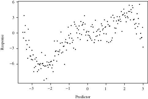
Consider the bivariate data shown in Figure 11.1. If asked, virtually anyone could draw a smooth curve that fits the data well, yet most would find it surprisingly difficult to describe precisely how they had done it. We focus here on a variety of methods for this task, called scatterplot smoothing.
Figure 11.1 Predictor–response data. A smooth curve sketched through these data would likely exhibit several peaks and troughs.

Effective smoothing methods for bivariate data are usually much simpler than for higher-dimensional problems; therefore we initially limit consideration to the case of n bivariate data points (xi, yi), i = 1, . . ., n. Chapter 12 covers smoothing multivariate data.
The goal of smoothing is different for predictor–response data than for general bivariate data. With predictor–response data, the random response variable Y is assumed to be a function (probably stochastic) of the value of a predictor variable X. For example, a model commonly assumed for predictor–response data is Yi = s (xi) + ![]() i, where the
i, where the ![]() i are zero-mean stochastic noise and s is a smooth function. In this case, the conditional distribution of Y|x describes how Y depends ...
i are zero-mean stochastic noise and s is a smooth function. In this case, the conditional distribution of Y|x describes how Y depends ...

