Digital Signal Processing Techniques and Applications in Radar Image Processing

2

DISCRETE TIME AND FREQUENCY TRANSFORMATION

This chapter addresses discrete signal transformations in both time and frequency domains. The relationship between continuous and discrete Fourier transform is discussed in Section 2.1. Section 2.2 reviews several key properties of discrete Fourier transform. The effect of Window functions on discrete Fourier transform is described in Section 2.3, and fast discrete Fourier transform techniques are covered in Section 2.4. The discrete cosine transform is reviewed in Section 2.5. Finally, the relationship between continuous and discrete signals in both time and frequency domains is illustrated graphically with an example in Section 2.6.

2.1 CONTINUOUS AND DISCRETE FOURIER TRANSFORM

It was shown in Chapter 1 that a periodic signal g_p(t) can be expressed as

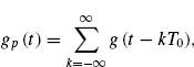
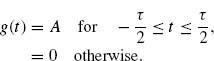
where T₀ is the period of g(t), and

It also was shown that g_p(t) can be represented in terms of Fourier series coefficients as

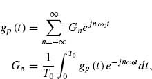
where ω₀ = 2π/T₀.

Now, let t = n ΔT and τ = N₁ ΔT, where ΔT = 1/f_s, and f_s is the sampling frequency that satisfies the Nyquist requirement. Assume that all frequencies are normalized with respect to f_s, or f_s = 1. Then t = nΔT = n, T₀ = NΔT = N, τ = N₁ΔT = N₁