Digital Signal Processing Using Matlab

4.2. Solved exercises

EXERCISE 4.1.

Consider 2,048 samples of a Gaussian white random process P with a unit mean value and a variance of 0.25. Check if it is a Gaussian random variable using different tests.

% Random process generation
P=0.5*randn(1,2048)+1;
mp = mean(P)
vp = var(P)

1^st test: the simplest test uses the random process histogram.

bins = 20;
hist(P,bins);

It can easily be seen that the obtained histogram is very similar to a Gaussian pdf.

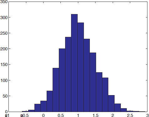
Figure 4.2. Histogram of a Gaussian random process

2^nd test: Let us calculate 3^rd and 4^th order cumulants of the random process P using equations [4.6] and [4.7].

Cum3 = mean(P.^3) - 3*mean(P)*mean(P.^2)+2* mean(P)^3
Cum4 = mean(P.^4) - 4*mean(P)*mean(P.^3) - 3*mean(P.^2)^2 +
12*mean(P)^2*mean(P.^2)- 6*mean(P)^4

Cum3 =
   0.0234

Cum4 =
   0.0080

The obtained values for the two cumulants are close to zero, so the Gaussianity hypothesis on P is reinforced.

3^rd test: Henry line.

nb_bins = 20;
[hv,x]=hist(P,nb_bins);
F=cumsum(hv)/sum(hv); F(end)=0.999 ;% empirical cdf
y=norminv(F,0,1); % percentile of a N(0,1) distributed variable
% Graphical matching
p=polyfit(x,y,1); % linear matching of x and y
s=1/p(1) % standard deviation estimation = inverse of the slope
z=polyval(p,x); % values on the Henry line
figure;
hold on;
plot(x,z,'-r');
plot (x,y,'*');
legend.('Henry line', 'Couples (x,t)');
xlabel('x');
ylabel('t');

Figure 4.3. Henry ...