book

Feedback Control for Computer Systems

by Philipp K. Janert

October 2013

Intermediate to advanced

330 pages

7h 46m

English

O'Reilly Media, Inc.

Read now

Unlock full access

What Is Feedback?Why This Book?How to Read This BookConventions Used in This BookUsing Code ExamplesSafari® Books OnlineHow to Contact UsAcknowledgments
A Hands-On ExampleHoping for the BestEstablishing ControlAdding It UpSummaryCode to Play With
Systems and SignalsTracking Error and Corrective ActionStability, Performance, Accuracy The SetpointUncertainty and Change Feedback and FeedforwardFeedback and Enterprise SystemsCode to Play With
Lags and Delays Forced Response and Free Response Transient Response and Steady-State ResponseDynamics in the Physical World and in the Virtual World Dynamics and MemoryThe Importance of Lags and Delays for Feedback Loops Avoiding DelaysTheory and PracticeCode to Play With
Block DiagramsOn/Off ControlProportional Control Why Proportional Control Is Not EnoughIntegral Control Integral Control Changes the Dynamics Integral Control Can Generate a Constant OffsetDerivative Control Problems with Derivative ControlThe Three-Term or PID ControllerCode to Play With
Control Input and Output Directionality of the Input/Output RelationExamples Thermal Control 1: HeatingSituationInputOutputCommentary Item CacheSituationInputOutputCommentary Server ScalingSituationInputOutputCommentary Controlling Supply and Demand by Dynamic PricingSituationInputOutputCommentary Thermal Control 2: CoolingSituationInputOutputCommentaryCriteria for Selecting Control Signals For Control Inputs For Control OutputsA Note on Multidimensional Systems
The Feedback IdeaIterationProcess KnowledgeAvoiding InstabilityThe SetpointControl, Not Optimization
Frequency RepresentationThe Transfer FunctionBlock-Diagram AlgebraPID ControllersPoles of the Transfer FunctionProcess Models

Static Input/Output Relation: The Process Characteristic Practical ConsiderationsDynamic Response to a Step Input: The Process Reaction Curve Practical AspectsProcess Models Self-Regulating Process Accumulating Process Self-Regulating Process with Oscillation Non-Minimum Phase SystemOther Methods of System Identification
Tuning ObjectivesGeneral Effect of Changes to Controller ParametersZiegler–Nichols TuningSemi-Analytical Tuning Methods Practical AspectsA Closer Look at Controller Tuning Formulas
Actuator Saturation and Integrator Windup Preventing Integrator Windup Setpoint Changes and Integrator PreloadingSmoothing the Derivative TermChoosing a Sampling IntervalVariants of the PID Controller Incremental Form Error Feedback Versus Output Feedback The General Linear Digital ControllerNonlinear Controllers Error-Square and Gap Controllers Simulating Floating-Point Output Categorical Output
Changing Operating Conditions: Gain Scheduling Gain Scheduling for Mildly Nonlinear SystemsLarge Disturbances: FeedforwardFast and Slow Dynamics: Nested or “Cascade” ControlSystems Involving Delays: The Smith Predictor
The Case StudiesModeling Time Control Time Simulation TimeThe Simulation Framework Components Plants and Systems Controllers Actuators and Filters Convenience Functions for Standard Loops Generating Graphical Output
Defining Components Cache Misses as Manufacturing DefectsMeasuring System CharacteristicsController TuningSimulation Code
The SituationMeasuring System CharacteristicsEstablishing ControlImproving PerformanceVariations Cumulative Goal Gain Scheduling Integrator Preloading Weekend EffectsSimulation Code
The SituationMeasuring and TuningReaching 100 Percent With a Nonstandard ControllerDealing with LatencySimulation Code
On the Nature of Queues and BuffersThe ArchitectureSetup and TuningDerivative Control to the RescueController AlternativesSimulation Code
The SituationThe ModelTuning and CommissioningClosed-Loop PerformanceSimulation Code
The SituationProblem AnalysisArchitecture Alternatives A Nontraditional Loop Arrangement A Traditional Loop with LogarithmsResultsSimulation Code
Simple Controllers, Simple LoopsMeasuring and TuningStaying in ControlDealing with Noise
Differential EquationsLaplace Transforms Properties of the Laplace TransformUsing the Laplace Transform to Solve Differential Equations A Worked ExampleThe Transfer Function Worked Example: Step Response Worked Example: Ramp Input The Harmonic OscillatorWhat If the Differential Equation Is Not Known?
Composite SystemsThe Feedback Equation An Alternative Derivation of the Feedback EquationBlock-Diagram AlgebraLimitations and Importance of Transfer Function Methods
The Transfer Function of the PID ControllerThe Canonical Form of the PID ControllerThe General ControllerProportional Droop Revisited A Worked Example
Structure of a Transfer FunctionEffect of Poles and Zeros Special Cases and Additional DetailsComplex conjugate polesMultiple polesPoles on the imaginary axisPole/zero cancellationsPole Positions and Response Patterns Dominant Poles Pole PlacementWhat to Do About Delays
Construction of Root Locus DiagramsRoot Locus or “Evans” RulesAngle and Magnitude CriteriaPractical IssuesExamples Simple Lag with a P Controller Simple Lag with a PI Controller
Frequency Response Frequency Response in the Physical World Frequency Response for Transfer Functions A Worked ExampleThe Bode PlotA Criterion for Marginal StabilityOther Graphical Techniques
Discrete-Time Modeling and the z-TransformState-Space MethodsRobust ControlOptimal ControlMathematical Control Theory
Basic PlottingPlot RangesInline TransformationsPlotting Simulation ResultsSummary
Basic OperationsPolar CoordinatesThe Complex Exponential
Recommended ReadingAdditional ReferencesMathematical Prerequisites

Content preview from Feedback Control for Computer Systems

Chapter 20. The Transfer Function

As Chapter 3 demonstrated, understanding a system’s dynamic behavior is important for building a stable and well-performing feedback loop. In this chapter, we will first describe how to capture information on a system’s dynamic behavior; we then show how to repackage this information in a way that is particularly convenient for our purposes. The tool that we will use is the transfer function.

Differential Equations

The usual way to describe the time evolution of a system is through differential equations. A differential equation is an expression involving the derivative of a quantity, often together with the quantity itself. Here are some examples of differential equations:

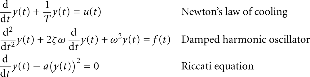
Because the derivative is the rate of change of the quantity, differential equations are the natural way to describe how a system changes over time: they describe the system’s dynamics. “Solving” a differential equation means finding a curve y(t) that, for all times t, fulfills the differential equation. Several analytical and numerical methods exist to find the solution to a given differential equation.

Laplace Transforms

Differential equations provide an especially compact way of describing the dynamics of a system: all possible trajectories, for all times t, can be obtained from the differential equation alone.^[21] We now repackage this information in a way that makes it easier ...