Growth Curve Modeling: Theory and Applications

4

ESTIMATION OF TREND

4.1 LINEAR TREND EQUATION

Let us consider what we shall call a purely mathematical (linear) model involving Y as a function of time t or

where β₀ is the (constant) vertical intercept and β₁ is the (constant) slope. Here β₀ is the value of Y when t = 0 while β₁ = ΔY/Δt (=rise/run). Specifically, β₁ is the rate of change in Y per unit change in t. So if β₁ = 5, then when t increases by one unit, Y increases by five units; and if β₁ = −3, then as t increases by one unit, Y decreases by three units.

To obtain Equation 4.1, we need only two specific points in the (t, Y)-plane (Fig. 4.1). That is, β₁ = ΔY/Δt = (Y₂ − Y₁)/(t₂ − t₁); and at, say, (t₂,Y₂), β₀ = Y − β₁t = Y₂ − β₁t₂. For instance, suppose (t₁, Y₁) = (1, 2) and (t₂, Y₂) = (4, 7). What is the equation of the line passing through these two points?

Clearly β₁ = ΔY/Δt = (7 − 2)/(4 − 1) = 5/3 while, at (t₁, Y₁), β₀ = 2 − (5/3)(1) = 1/3. Hence our particularization of Equation 4.1 is Y = (1/3) + (5/3)t. So when, t = 0, Y = 1/3; and, for β₁ = 5/3, when t increases by one unit, Y increases by 5/3 units.

What if we have more than two points in the (t, Y)-plane? Specifically, we may have a scatter of points such as the one depicted in Figure 4.2.

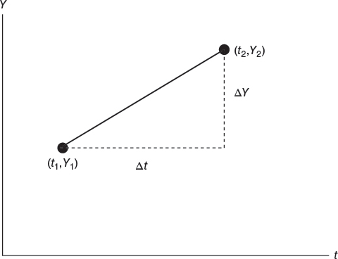
FIGURE 4.1 The line through the points (t₁,Y₁) and (t₂,Y₂).

FIGURE ...