Introduction to Mixed Modelling: Beyond Regression and Analysis of Variance, 2nd Edition

10.10 A more general pattern in the covariance matrix: Analysis of pedigrees and genetic data

In all the mixed models we have considered so far, the covariance matrix for each term is of the form shown in Equation 10.27 – an identity matrix, having 1s along the leading diagonal and 0s elsewhere, multiplied by the variance component for the term in question. However, the covariance matrix need not be so simple: we have already seen an instance of non-zero covariance between two random-effect terms, namely the slopes and intercepts in the random-coefficient model (Sections 7.5–7.7; see also Exercise 10.3 at the end of this chapter). For an example of non-zero covariances within a single term, consider the pedigree in Figure 10.8, which represents three generations of animals. Earlier generations are represented in higher rows of the pedigree: animals represented in the bottom row are the most recent generation, those in the row above are their parents and those in the top row their grandparents.

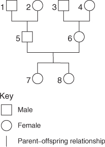
Figure 10.8 A pedigree representing three generations of animals.

Suppose that a continuous variable Y (e.g. weight) is measured on each animal in this pedigree, and that this variable comprises a genetic effect Γ and an environmental effect Ε, so that

10.28

where

1. μ = the mean value ...