Modern Control System Theory and Design, 2nd Edition

2.30  ILLUSTRATIVE PROBLEMS AND SOLUTIONS

This section provides a set of illustrative problems and their solutions to supplement the material presented in Chapter 2.

I2.1. Determine the poles and zeros of

SOLUTION: Simple poles are located at s = 0, −2, −6

Pole of order two located at −8

Simple zeros located at −1, −4

I2.2. Determine the Laplace transform of f(t) which is given by

f(t) = te^4t,   t ≥0

f(t) = 0,      t > 0.

SOLUTION: From Appendix A, eighth item: For n = 2 and a = −4, we obtain

I2.3. Determine the Laplace transform F(s) for the function f(t) illustrated:

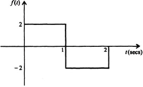
Figure I2.3

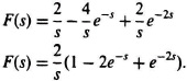
SOLUTION:

f(t) = 2U(t) − 4U(t − 1) + 2U(t − 2)

From Table 2.1, item 2, and the time-shifting theorem, we obtain

I2.4. Determine the initial value of c(t) where the Laplace transform of C(s) is given by:

SOLUTION: From the initial-value theorem

we obtain,

I2.5. Determine the final value of c(t) when the Laplace ...