Physically Based Rendering, 3rd Edition

14.5: Path tracing

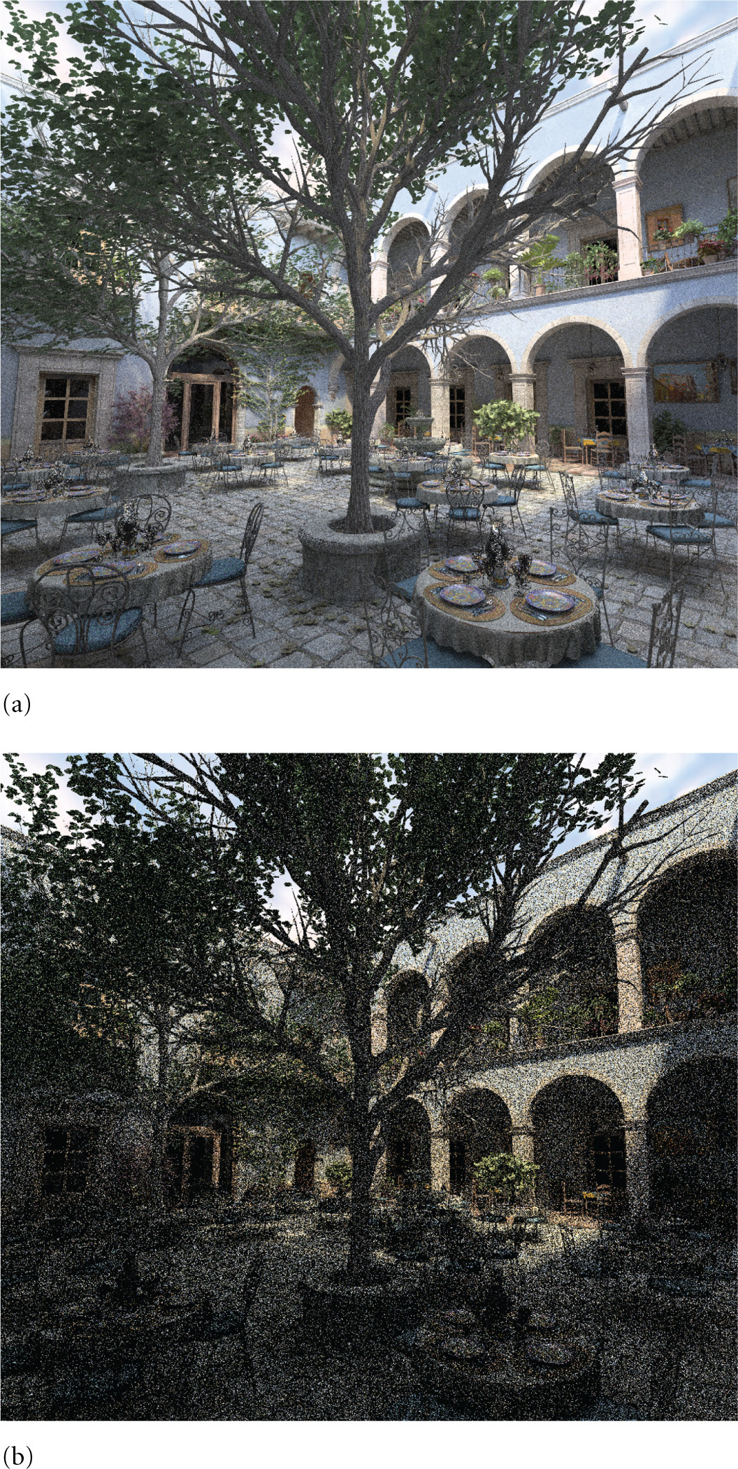
Now that we have derived the path integral form of the light transport equation, we’ll show how it can be used to derive the path-tracing light transport algorithm and will present a path-tracing integrator. Figure 14.17 compares images of a scene rendered with different numbers of pixel samples using the path-tracing integrator. In general, hundreds or thousands of samples per pixel may be necessary for high-quality results—potentially a substantial computational expense.

Figure 14.17 San Miguel Scene Rendered with Path Tracing. (a) Rendered with path tracing with 1024 samples per pixel. (b) Rendered with just 8 samples per pixel, ...