Practical Automated Machine Learning on Azure

Chapter 1. Machine Learning: Overview and Best Practices

How are humans different from machines? There are quite a few differences, but here’s an important one: humans learn from experience, whereas machines follow instructions given to them. What if machines can also learn from experience? That is the crux of machine learning. For machines, “data from the past” is the logical equivalent of “experience.” Machine learning combines statistics and computer science to enable machines to learn how to perform a given task without being explicitly programmed to do so via instructions.

Machine learning is widely used today, and we interact with it every day. Here are a few examples to illu strate:

• Search engines like Bing or Google

• Product recommendations at online stores like Amazon or eBay

• Personalized video recommendations at Netflix or YouTube

• Voice-based digital assistants like Alexa or Cortana

• Spam filters for our email inbox

• Credit card fraud detection

Why is machine learning as a trend emerging so fast? Why is everyone so interested in it now? As shown in Figure 1-1, its popularity arises from three key trends: big data, better/cheaper compute, and smarter algorithms.

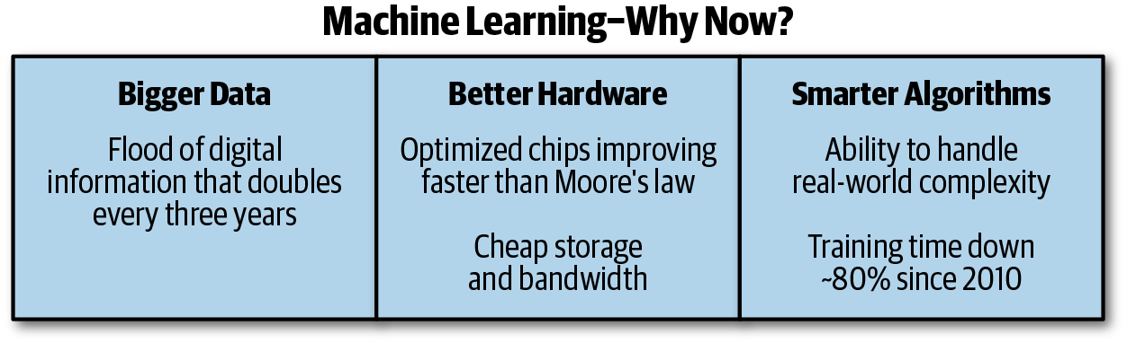
Figure 1-1. Machine learning growth

In this chapter, we provide a quick refresher on machine learning by using a real-world example, discuss some of the best practices that differentiate successful machine learning projects from the rest, and end with challenges around productivity and scale.

Machine Learning: A Quick Refresher

What does the process of building a machine learning model look like? Let’s dig deeper using a real scenario: house price prediction. We have past home sales data, and the task is to predict the sale price for a given house that just came onto the market and isn’t currently in our dataset.

For simplicity, let’s assume that the size of the house (in square feet) is the most important input attribute (or feature) that determines house value. As shown in Table 1-1, we have data from four houses, A, B, C, D, and we need to predict the price of house X.

Table 1-1. House prices based on size

House	Size (sq. ft)	Price ($)
A	1300	500,000
B	2000	800,000
C	2500	950,000
D	3200	1,200,000
X	1800	?

We begin by plotting Size on the x-axis and Price on the y-axis, as shown in Figure 1-2.

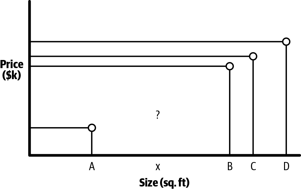
Figure 1-2. Plotting price versus size

What’s the best estimate for the price of house X?

• $550,000

• $700,000

• $1,000,000

Let’s figure it out. As shown in Figure 1-3, the four points that we plotted based on the data form an almost straight line. If we draw this line that best fits our data, we can find the right point on the line associated with house X on the x-axis and the corresponding point on y-axis, which will give us our price estimate.

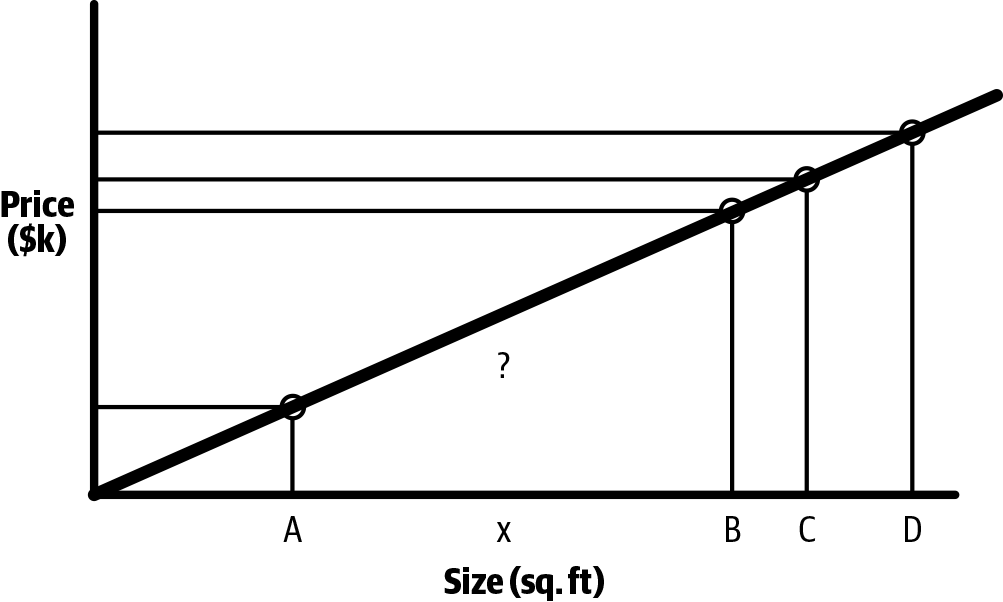
Figure 1-3. Creating a straight line to find price estimate

In this case, that straight line represents our model—and demonstrates a linear relationship. Linear regression is a statistical approach for modeling a linear relationship between input variables (also called feature, or independent, variables) and an output variable (also called a target, or dependent, variable). Mathematically, this linear relationship can be represented as follows:

$$y=\mathit{\beta 0}+\mathit{\beta 1x}$$

where:

• y is the output variable; for example, the house price.

• x is the input variable; for example, size in square feet.

• β0 is the intercept (the value of y when x = 0).

• β1 is the coefficient for x and the slope of the regression line (“the average increase in y associated with a one-unit increase in x).

Model Parameters

β0 and β1 are known as the model parameters of this linear regression model. When implementing linear regression, the algorithm finds the line of best fit by using the model parameters β0 and β1, such that it is as close as possible to the actual data points (minimizing the sum of the squared distances between each actual data point and the line representing model predictions).

Figure 1-4 shows this conceptually. Dots represent actual data points, and the line represents the model predictions. d1 to d9 represent distances between data points and the corresponding model prediction, and D is the sum of their squares. The line shown in the figure is the best-fit regression line that minimizes D.

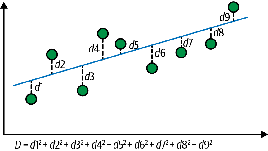
Figure 1-4. Regression

As you can see, model parameters are an integral part of the model and determine the outcome. Their values are learned from data through the model training process.

Hyperparameters

There is another set of parameters known as hyperparameters. Model hyperparameters are used during the model training process to establish the correct values of model parameters. They are external to the model, and their values cannot be estimated from data. The choice of the hyperparameters will affect the duration of the training and the accuracy of the predictions. As part of the model training process, data scientists usually specify hyperparameters based on heuristics or knowledge, and often tune the hyperparameters manually. Hyperparameter tuning relies more on experimental results than theory, and thus the best method to determine the optimal settings is to try many combinations and evaluate the performance of each model.

Simple linear regression doesn’t have any hyperparameters. But variants of linear regression, like Ridge regression and Lasso, do. Here are some examples of model hyperparameters for various machine learning algorithms:

• The k in k-nearest neighbors

• The desired depth and number of leaves in a decision tree

• The C and sigma in support vector machines (SVMs)

• The learning rate for a neural network training

Best Practices for Machine Learning Projects

In this section, we examine best practices that make machine learning projects successful. These are practical tips that most companies and teams end up learning with experience.

Understand the Decision Process

Machine learning–based systems or processes use data to drive business decisions. Hence, it is important to understand the business problem that needs to be solved, independent of technology solutions—in other words, what decision or action needs to be taken that can be informed by data. Being clear about the decision process is critical. This step is also sometimes referred to as mapping a business scenario/problem to a data science question.

For our house-price prediction scenario, the key business decision for a home buyer, is “Should I buy a given house at the listed price?” or “What is a good bid price for this house to maximize my chance of winning the bid?” This could be mapped to the data science question: “What is the best estimate of the house price based on past sales data of other houses?”

Table 1-2 shows other real-world business scenarios and what this decision process looks like.

Table 1-2. Understanding a decision process: real-world scenarios

Business scenario	Key decision	Data science question
Predictive maintenance	Should I service this piece of equipment?	What is the probability this equipment will fail within the next x days?
Energy forecasting	Should I buy or sell energy contracts?	What will be the long-/short-term demand for energy in a region?
Customer churn	Which customers should I prioritize to reduce churn?	What is the probability of churn within x days for each customer?
Personalized marketing	What product should I offer first?	What is the probability that customers will purchase each product?
Product feedback	Which service/product needs attention?	What is the social media sentiment for each service/product?

Establish Performance Metrics

As with any project, performance metrics are important to guide any machine learning project toward the proper goals and to ensure progress is made. After we understand the decision process, the next step is to answer these two key questions:

• How do we measure progress toward a goal or desired outcome? In other words, how do we define metrics to evaluate progress?

• What would be considered a success? That is, how do we define targets for the metrics defined?

For our house-price prediction example, we need a metric to measure how close our predictions are to the actual price. There are quite a few metrics to choose from. One of the most commonly used metrics for regression tasks is root-mean-square error (RMSE). This is defined as the square root of the average squared distance between the actual score and the predicted score, as shown here:

$$\text{RMSE}=\sqrt{\frac{1}{n}{\sum }_{j=1}^n{(y_j-{\widehat{y}}_j)}^2}$$

Here, y_j denotes the true value for the i^th data point, and ŷ_j denotes the predicted value. One intuitive way to understand this formula is that it is the Euclidean distance between the vector of the true values and the vector of the predicted values, averaged by n, where n is the number of data points.

Focus on Transparency to Gain Trust

There is a common perception that machine learning is a black box that just works magically. It is critical to understand that although model performance as measured by metrics is important, it is even more important for us to understand how the model works. Without this understanding, it is difficult to trust the model and therefore difficult to convince key stakeholders and customers of the business value of machine learning and machine learning–based systems.

In heavily regulated industries like health care and banking, which are required to comply with regulation, interpretability of models is critical. Model interpretability is typically represented by feature importance, which tells you how each input column (or feature) affects the model’s predictions. This allows data scientists to explain resulting predictions so that stakeholders can see which data points are most important in the model.

In our house-price prediction scenario, our trust on the model would increase if the model, in addition to price prediction, indicated key input features that contributed to the output; for example, house size and age. Figure 1-5 shows feature importance for our house-price prediction scenario. Notice that age and school rating are the topmost features.

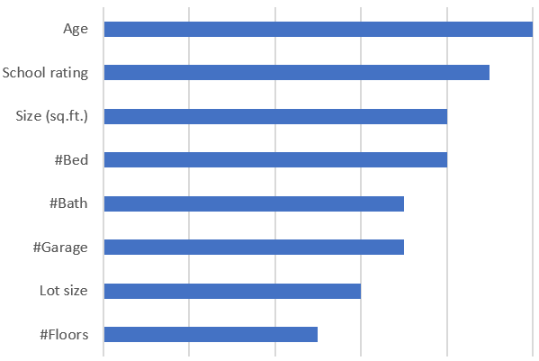
Figure 1-5. Feature importance

Embrace Experimentation

Building a good machine learning model takes time. As with other software projects, the trick to becoming successful in machine learning projects lies in how fast we try out new hypotheses, learn from them, and keep evolving. As shown in Figure 1-6, the path to success isn’t usually easy and requires a lot of persistence, due diligence, and failures on the way.

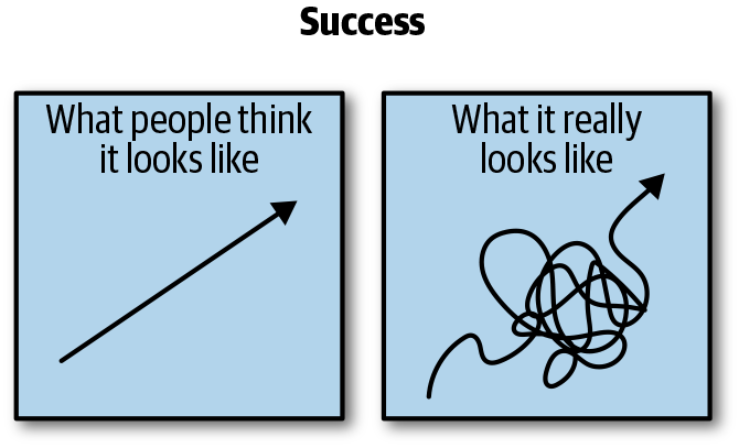
Figure 1-6. Success is not easy.

Here are key aspects of a culture that values experimentation:

• Be willing to learn from experiments (successes or failures).

• Share the learning with peers.

• Promote successful experiments to production.

• Understand that failure is a valid outcome of an experiment.

• Quickly move on to the next hypothesis.

• Refine the next experiment.

Don’t Operate in a Silo

Customers typically experience machine learning models through applications. Figure 1-7 shows how machine learning systems are different from traditional software systems. The key difference is that machine learning systems, in addition to code workflow, must also consider data workflow.

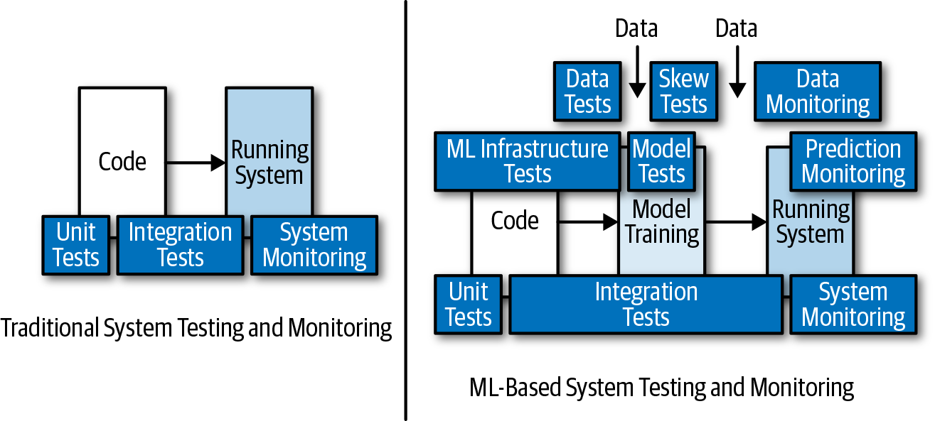
Figure 1-7. Machine learning system versus traditional systems

After data scientists have built a machine learning model that is satisfactory to them, they hand it off to an app developer who integrates it into the larger application and deploys it. Often, any bugs or performance issues go undiscovered until the application has already been deployed. The resulting friction between app developers and data scientists to identify and fix the root cause can be a slow, frustrating, and expensive process.

As machine learning enters more business-critical applications, it is increasingly clear that data scientists need to collaborate closely with app developers to build and deploy machine learning–powered applications more efficiently. Data scientists are focused on the data science life cycle; namely, data ingestion and preparation, model building, and deployment. They are also interested in periodically retraining and redeploying the model to adjust for freshly labeled data, data drift, user feedback, or changes in model inputs. The app developer is focused on the application life cycle—building, maintaining, and continuously updating the larger business application that the model is part of. Both parties are motivated to make the business application and model work well together to meet end-to-end performance, quality, and reliability goals.

What is needed is a way to bridge the data science and application life cycles more effectively. Figure 1-8 shows how this collaboration could be enabled. We will cover this in more depth later in the book.

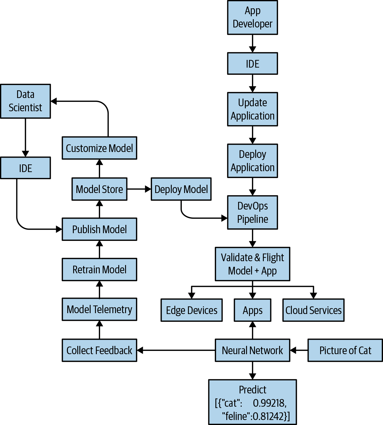
Figure 1-8. App developer and data scientist working together

An Iterative and Time-Consuming Process

In this section, we dig deeper into the machine learning process by using our house-price prediction example. We started with house size as the only input, and we saw the relationship between house size and house price to be linear. To create a good model that can predict prices more accurately, we need to explore good input features, select the best algorithm, and tune hyperparameter values. But, how do you know which features are good, and which algorithm and hyperparameter values will do the best? There is no silver bullet here; we will need to try out different combinations of features, algorithms, and hyperparameter values. Let’s take a look at each of these three steps and then see how they apply to our house-price prediction problem.

Feature Engineering

Feature engineering is the process of using our knowledge of the data to create features that make machine learning algorithms work. As shown in Figure 1-9, this involves four steps.

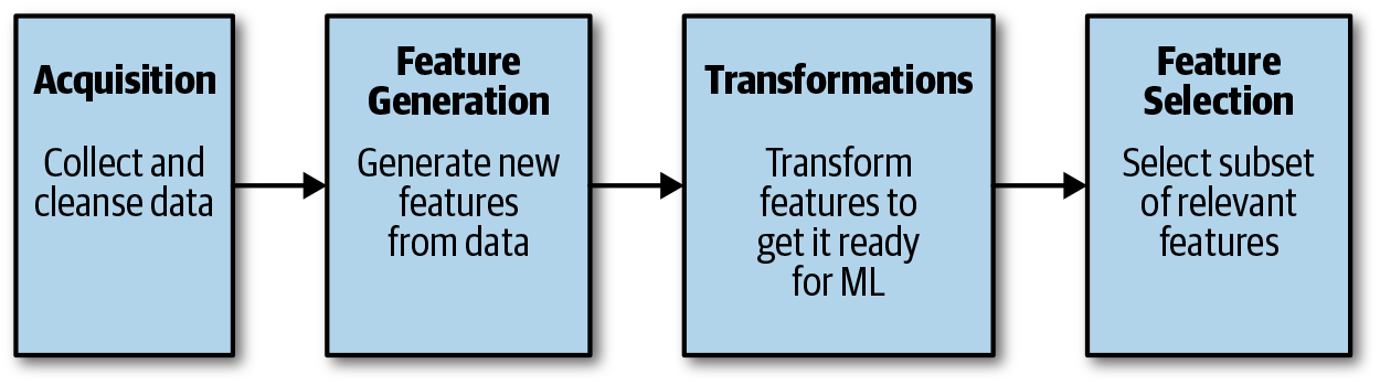
Figure 1-9. Feature engineering

First, we acquire data—collect the data with all of these possible input variables/features and get it to a usable state. Most real-world datasets are not clean, and need work to get the data to a level of quality before using it. This can involve things such as fixing missing values, removing anomalies and possibly incorrect data, and ensuring the data distribution is representative.

Next you’ll need to generate features: explore generating more features from available data. This is typically useful when dealing with text data or time-series data. Text-related features could be as simple as n-grams and count vectorization or as advanced as sentiment from review text. Similarly, time-related features could be as simple as month and week-index-of-year or as complex as time-based aggregations. These additional features generated can prove helpful in improving accuracy of the model.

With this complete, you’ll need to transform the data to make it suitable for machine learning. Often, machine learning algorithms require that data be prepared in specific ways before fitting a machine learning model. For instance, many such algorithms cannot operate on categorical data directly, and require all input variables and output variables be numeric. A categorical variable is a variable that can take on one of a limited, and usually fixed, number of possible values. Examples of these variables include color (red, blue, green, etc.), country (United States, India, China, etc.), and blood group (A, B, O, AB). Categorical variables must be converted to a numerical form, which is typically done by using integer encoding or one-hot encoding techniques.

The final step is feature selection: choosing a subset of features to train the model on. Why is this necessary? Why not train the model with the full set of features? Feature selection identifies and removes the unneeded, irrelevant, and redundant attributes from data that don’t contribute, or can in fact decrease, the model’s accuracy. The objective of feature selection is threefold:

• Improve model accuracy

• Improve model training time/cost

• Provide a better understanding of the underlying process of feature generation

Note

Feature engineering steps are critical for traditional machine learning but not so much for deep learning, because features are automatically generated/inferred through the deep learning network.

We began with a single feature: house size. But we know that the price of a house is dependent not only on size, but also on other characteristics. What other input features could influence house price? Although size might be one of the most important inputs, here are few more worth considering:

• Zip code

• Year built

• Lot size

• Schools

• Number of bedrooms

• Number of bathrooms

• Number of garage stalls

• Amenities

Algorithm Selection

After we have chosen a good set of features, the next step is to determine the correct algorithm for the model. For the data we have, a simple linear regression model might seem to work. But remember that we have only a few data points (four houses with price)—small enough to be representative and small enough for machine learning. Also, linear regression assumes a linear relation between input features and target variable. As we collect more data points, linear regression might not remain most relevant, and we will be motivated to explore other techniques (algorithms) depending on trends and patterns in data.

Hyperparameter Tuning

As discussed earlier in this chapter, hyperparameters play a key role in model accuracy and training performance. Hence, tuning them is a critical step in getting to a good model. Because different algorithms have different sets of hyperparameters, this step of tuning hyperparameters adds to the complexity of the end-to-end process.

The End-to-End Process

With that basic understanding of feature engineering, algorithm selection, and hyperparameter tuning, let’s go step by step through our house-price prediction problem.

Let’s begin with Size, Lot size, and Year built features and Gradient Boosted trees with specific hyperparameter values, as shown in Figure 1-10. The resulting model is 30% accurate. But we want to do better than that.

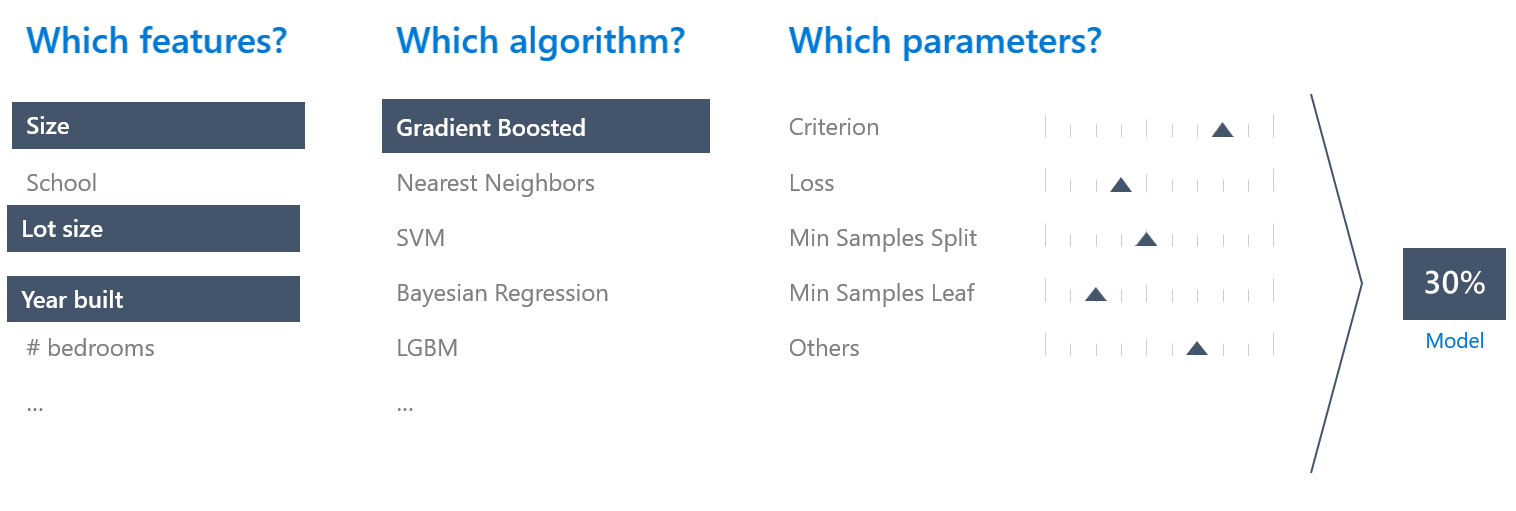
Figure 1-10. Machine learning process: step 1

To get underway, we try different values of hyperparameters for the same set of features and algorithm. If that doesn’t improve accuracy of the model to a satisfactory level, we try different algorithms, and if that doesn’t help either, we add more features. Figure 1-11 shows one such intermediate state, with School added as a feature and the k-nearest neighbors (KNN) algorithm used. The resulting model is 50% accurate but still not good enough, so we continue this process and try different combinations.

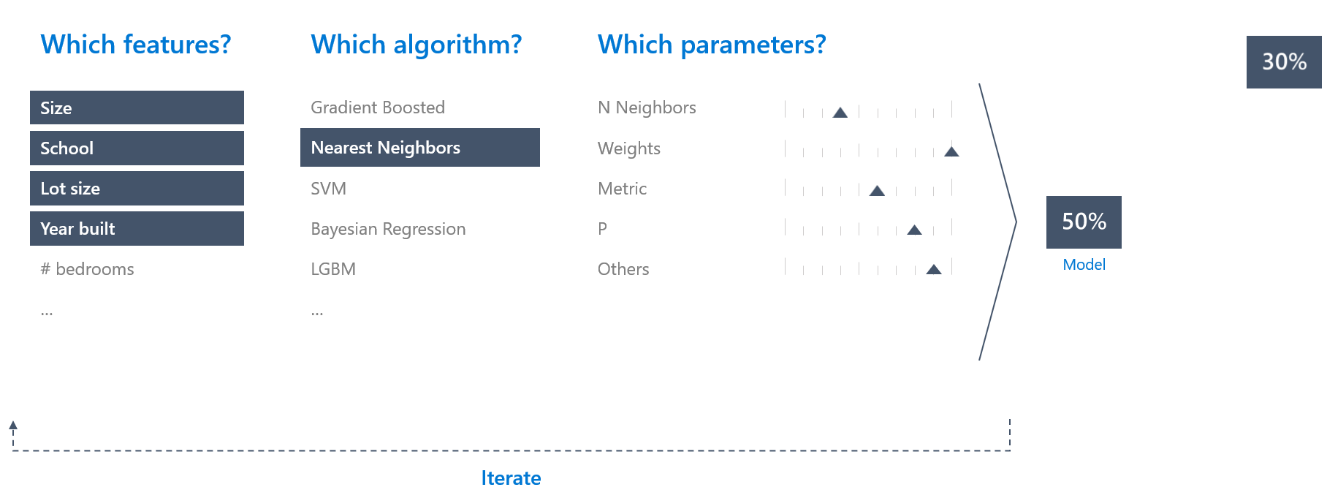
Figure 1-11. Machine learning process: intermediate state

After multiple iterations of trying out different combinations of features, algorithms, and hyperparameter values, we end up with a model that meets our criteria, as shown in Figure 1-12.

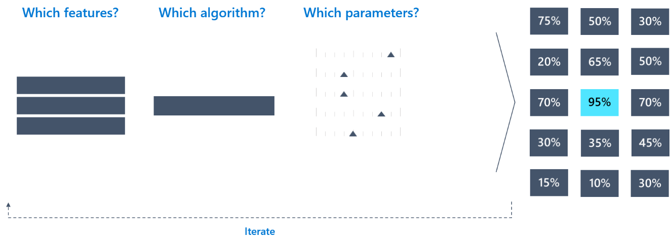
Figure 1-12. Machine learning process: best model

As you can see, this is an iterative and time-consuming process. To put this in perspective: if there are 10 features, there are a total of 2¹⁰ (1,024) ways to select features. If we try five algorithms, and assuming each has an average of five hyperparameters, we are looking at a total of 1,024 × 5 × 5 = 25,600 iterations!

Figure 1-13 shows the scikit-learn cheat sheet demonstrating that choosing the proper algorithm could be a complex problem in itself. Now imagine adding feature engineering and hyperparameter tuning on top of it. As a result, it takes data scientists anywhere from a couple of weeks to months to arrive at a good model.

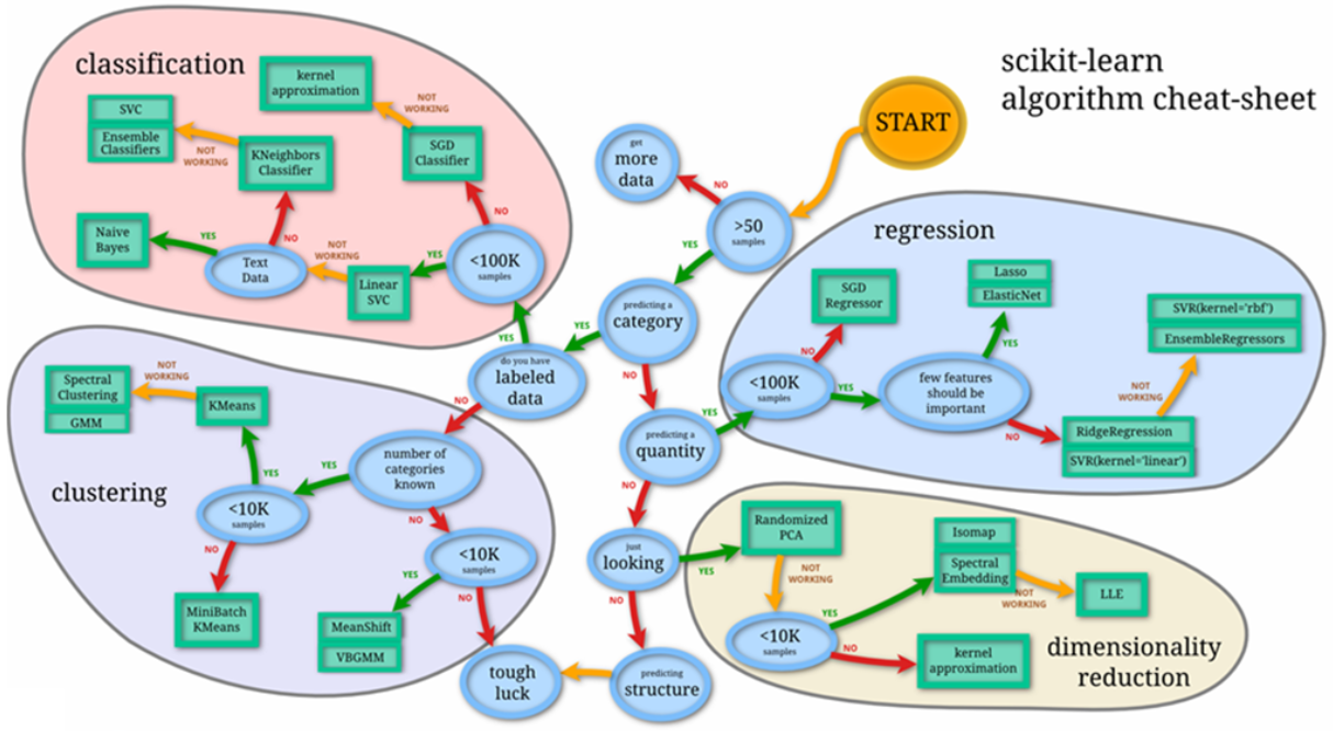
Figure 1-13. Scikit-learn algorithm cheat sheet (source: https://oreil.ly/xUZbU)

Growing Demand

Despite the complexity of the model-building process, demand for machine learning has skyrocketed. Most organizations across all industries are trying to use data and machine learning to gain a competitive advantage—infusing intelligence into their products and processes to delight customers and amplify business impact. Figure 1-14 shows the variety of real-world business problems being solved using machine learning.

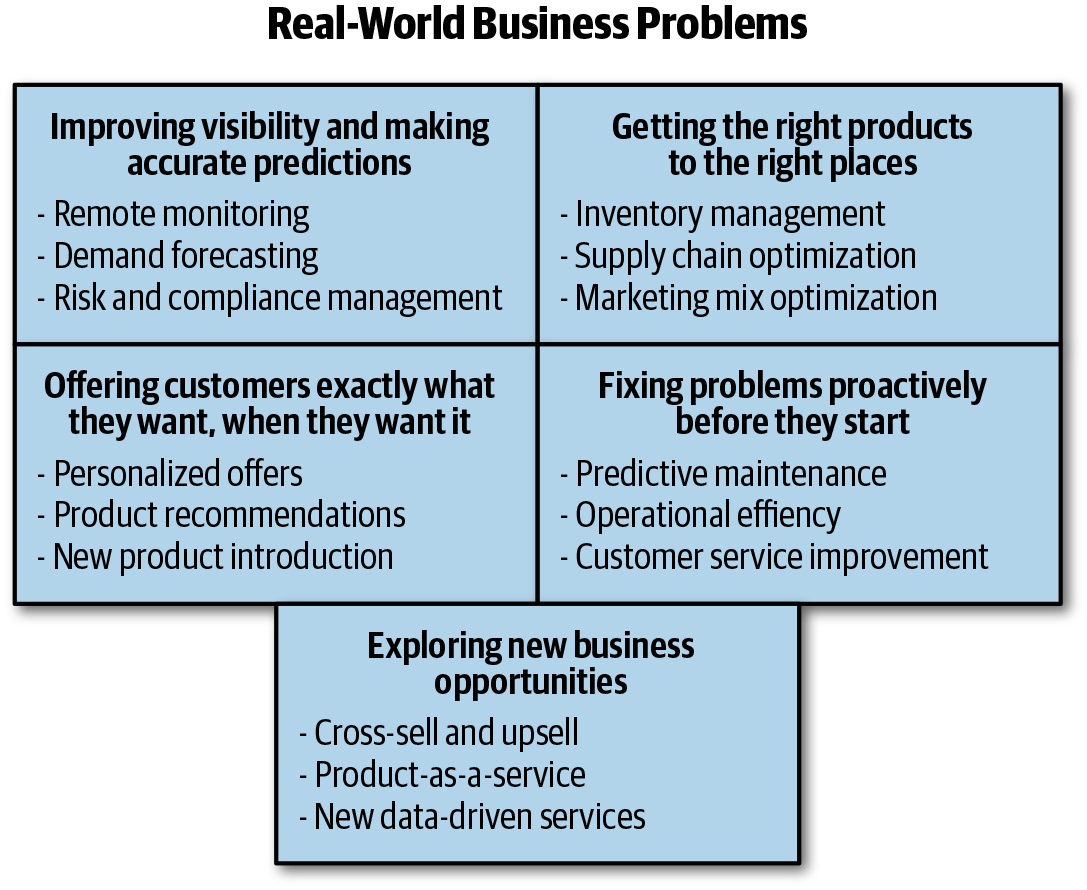
Figure 1-14. Real-world business problems using machine learning

As a result, there is huge demand for machine learning–related jobs. Figure 1-15 shows the percentage growth in various job postings from 2015 to 2018.

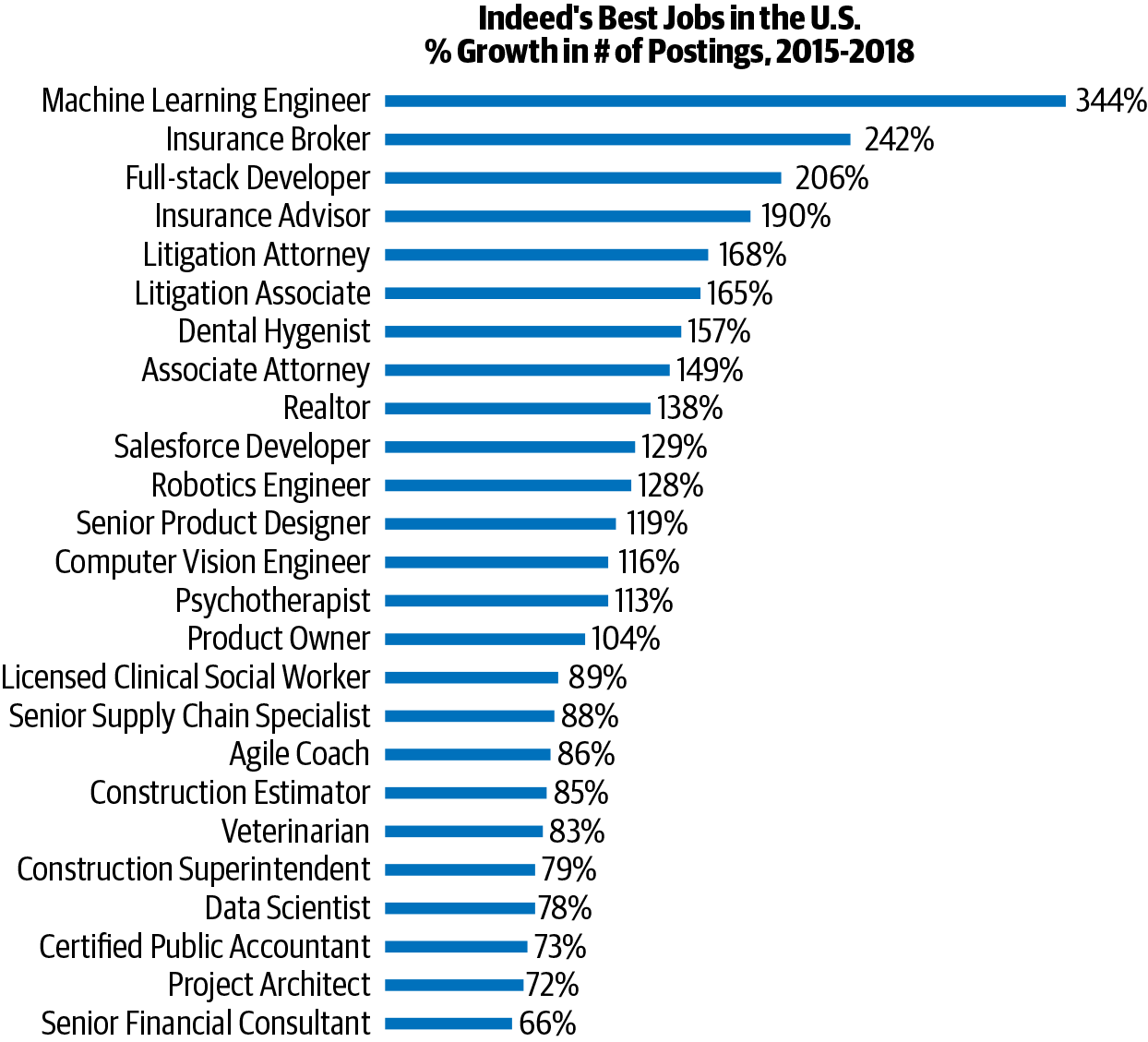
Figure 1-15. Growth in machine learning–related jobs

And Figure 1-16 shows the expected revenue from enterprise applications using machine learning and artificial intelligence growing astronomically.

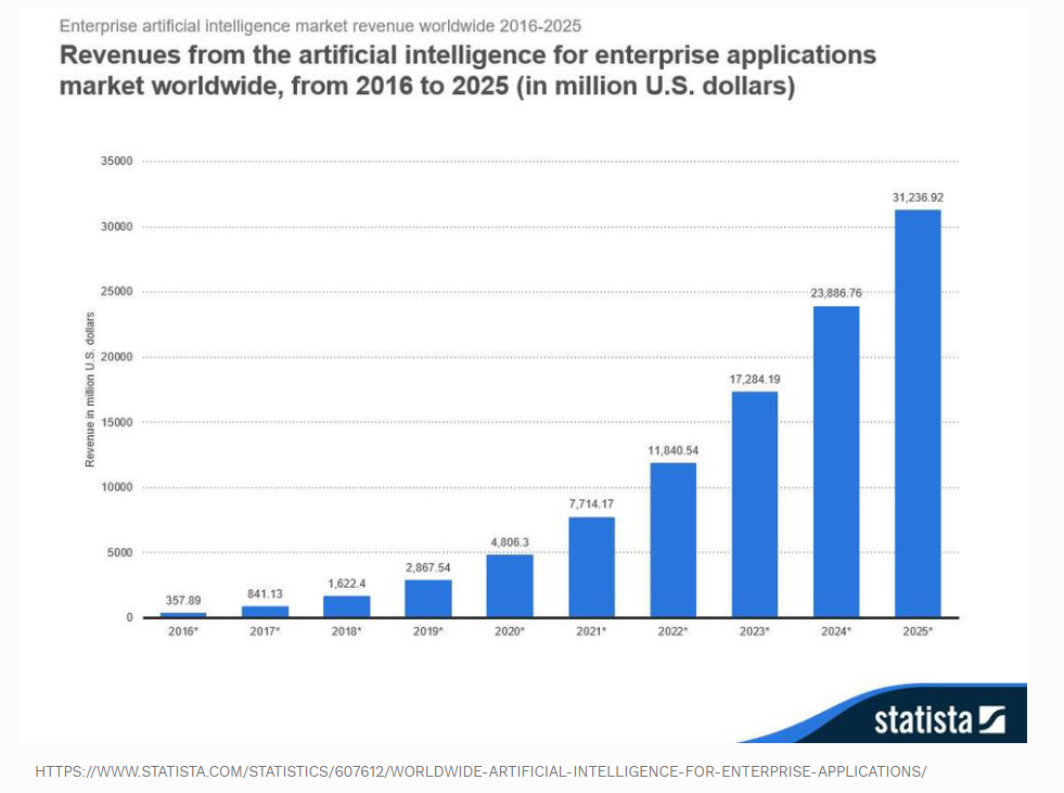
Figure 1-16. Machine learning/artificial intelligence revenue projections

Conclusion

In this chapter, you learned some of the best practices that successful machine learning projects have in common. We discussed that the process of building a good machine learning model is iterative and time-consuming, resulting in data scientists requiring anywhere from a couple of weeks to months to build a good model. At the same time, demand for machine learning is growing rapidly and is expected to skyrocket.

To balance this supply-versus-demand problem, there needs to be a better way to shorten the time it takes to build machine learning models. Can some of the steps in that workflow be automated? Absolutely! Automated Machine Learning is one of the most important skills that successful data scientists need to have in their toolbox for improved productivity.

In the following chapters we’ll go deeper into Automated Machine Learning. We will explore what it is, how to get started, and how it is being used in real-world applications today.