Practical Weak Supervision

Chapter 4. Using the Snorkel-Labeled Dataset for Text Classification

The key ingredient for supervised learning is a labeled dataset. Weakly supervised techniques provide machine learning practitioners with a powerful approach for getting the labeled datasets that are needed to train natural language processing (NLP) models.

In Chapter 3, you learned how to use Snorkel to label the data from the FakeNewsNet dataset. In this chapter, you will learn how to use the following Python libraries for performing text classification using the weakly labeled dataset, produced by Snorkel:

ktrain

At the beginning of this chapter, we first introduce the ktrain library. ktrain is a Python library that provides a lightweight wrapper for transformer-based models and enables anyone (including someone new to NLP) a gentle introduction to NLP.

Hugging Face

Once you are used to the different NLP concepts, we will learn how to unleash the powerful capabilities of the Hugging Face library.

By using both ktrain and pretrained models from the Hugging Face libraries, we hope to help you get started by providing a gentle introduction to performing text classification on the weakly labeled dataset before moving on to use the full capabilities of the Hugging Face library.

We included a section showing you how you can deal with a class-imbalanced dataset. While the FakeNewsNet dataset used in this book is not imbalanced, we take you through the exercise of handling the class imbalance to help you build up the skills, and prepare you to be ready when you actually have to deal with a class-imbalanced dataset in the future.

Getting Started with Natural Language Processing (NLP)

NLP enables one to automate the processing of text data in tasks like parsing sentences to extract their grammatical structure, extracting entities from documents, classifying documents into categories, document ranking for retrieving the most relevant documents, summarizing documents, answering questions, translating documents, and more. The field of NLP has been continuously evolving and has made significant progress in recent years.

Note

For a theoretical and practical introduction to NLP, the books Foundations of Natural Language Processing by Christopher D. Manning and Hinrich Schütze and Natural Language Processing with Python by Steven Bird, Ewan Klein, and Edward Loper will be useful.

Sebastian Ruder and his colleagues’ 2019 tutorial “Transfer Learning in Natural Language Processing”¹ will be a great resource to help you get started if you are looking to jumpstart your understanding of the exciting field of NLP. In the tutorial, Ruder and colleagues shared a comprehensive overview of how transfer learning for NLP works. Interested readers should view this tutorial.

The goal of this chapter is to show how you can leverage NLP libraries for performing text classification using a labeled dataset produced by Snorkel. This chapter is not meant to demonstrate how weak supervision enables application debugging or supports iterative error analsysis with the Snorkel model that is provided. Readers should refer to the Snorkel documentation and tutorials to learn more.

Let’s get started by learning about how transformer-based approaches have enabled transfer learning for NLP and how we can use it for performing text classification using the Snorkel-labeled FakeNewsNet dataset.

Transformers

Transformers have been the key catalyst for many innovative NLP applications. In a nutshell, a transformer enables one to perform sequence-to-sequence tasks by leveraging a novel self-attention technique.

Transformers use a novel architecture that does not require a recurrent neural network (RNN) or convolutional neural network (CNN). In the paper “Attention Is All You Need”, the authors showed how transformers outperform both recurrent and convolutional neural network approaches.

One of the popular transformer-based models, which uses a left/right language modeling objective, was described in the paper “Improving Language Understanding by Generative Pre-Training”. Over the last few years, Bidirectional Encoder Representations from Transformers (BERT) has inspired many other transformer-based models. The paper “BERT: Pre-training of Deep Bidirectional Transformers for Language Understanding” provides a good overview of how BERT works. BERT has inspired an entire family of transformer-based approaches for pretraining language representations. This ranges from the different sizes of pretrained BERT models (from tiny to extremely large), including RoBERTa, ALBERT, and more.

To understand how transformers and self-attention work, the following articles provide a good read:

“A Primer in BERTology: What We Know About How BERT Works”²

This is an extensive survey of more than 100+ studies of the BERT model.

“Transformers from Scratch” by Peter Bloem”³

To understand why self-attention works, Peter Bloem provided a good, simplified discussion in this article.

“The Illustrated Transformer” by Jay Alammar⁴

This is a good read on understanding how Transformers work.

“Google AI Blog: Transformer: A Novel Neural Network Architecture for Language Understanding”⁵

Blog from Google AI that provides a good overview of the Transformer.

Motivated by the need to reduce the size of a BERT model, Victor Sanh, Lysandre Debut, Julien Chaumond, and Thomas Wolf⁶ proposed DistilBERT, a language model that is 40% smaller and yet retains 97% of BERT’s language understanding capabilities. Consequently, this enables DistilBERT to perform at least 60% faster.

Many novel applications and evolutions of transformer-based approaches are continuously being made available. For example, OpenAI used transformers to create language models in the form of GPT via unsupervised pretraining. These language models are then fine-tuned for a specific downstream task.⁷ More recent transformer innovation includes GPT3 and Switch Transformers.

In this chapter, you will learn how to use the following transformer-based models for text classification:

• “DistilBERT, a Distilled Version of BERT: Smaller, Faster, Cheaper and Lighter”

• “RoBERTa: A Robustly Optimized BERT Pretraining Approach”

We will fine-tune the pretrained DistilBert and RoBERTa models and use them for performing text classification on the FakeNewsNet dataset. To help everyone jumpstart, we will start the text classification exercise by using ktrain. Once we are used to the steps for training transformer-based models (e.g., fine-tuning DistilBert using ktrain), we will learn how to tap the full capabilities of Hugging Face. Hugging Face is a popular Python NLP library, which provides a rich collection of pretrained models and more than 12,638 models (as of July 2021) on their model hub.

In this chapter, we will use Hugging Face for training the RoBERTa model and fine-tune it for the text classification task. Let’s get started!

Hard Versus Probabilistic Labels

In Chapter 3, we learned how we can use Snorkel to produce the labels for the dataset that will be used for training. As noted by the authors of the “Snorkel Intro Tutorial: Data Labeling”, the goal is to be able to leverage the labels from each of the Snorkel labeling functions and convert them into a single noise-aware probabilistic (or confidence-weighted) label.

In this chapter, we use the FakeNewsNet dataset and label that has been labeled by Snorkel in Chapter 3. This Snorkel label is referred to as a column, called snorkel_labels in the rest of this chapter.

Similar to the Snorkel Spam Tutorial, we will use snorkel.labeling.MajorityLabelVoter. The labels are produced by using the predict() method of snorkel.labeling.MajorityLabelVoter. From the documentation, the predict() method returns the predicted labels, which are returned as an ndarray of integer labels. In addition, the method supports different policies for breaking ties (e.g., abstain and random). By default, the abstain policy is used.

It is important to note that the Snorkel labeling functions (LFs) may be correlated. This might cause a majority-vote-based model to overrepresent some of the signals.

To address this, the snorkel.labeling.model.label_model.LabelModeL can be used. The predict() method of LabelModeL returns an ndarray of integer labels and an ndarray of probabilistic labels (if return_probs is set to True). These probabilistic labels can be used to train a classifier.

You can modify the code discussed in this chapter to use the probabilistic labels provided by LabelModel as well. Hugging Face implementation of transformers provide the BCEWithLogitsLoss function, which can be used with the probabilistic labels. (See the Hugging Face code for RoBERTa to understand the different loss functions supported.)

For simplicity, this chapter uses the label outputs from MajorityLabelVoter.

Using ktrain for Performing Text Classification

To help everyone get started, we will use the Python library ktrain to illustrate how to train a transformer-based model. ktrain enables anyone to get started with using a transformer-based model quickly. ktrain enables us to leverage the pretrained DistilBERT models (available in Hugging Face) to perform text classification.

Data Preparation

We load the fakenews_snorkel_labels.csv file and show the first few rows of the dataset:

import pandas as pd

# Read the FakeNewsNet dataset and show the first few rows
fakenews_df = pd.read_csv('../data/fakenews_snorkel_labels.csv')
fakenews_df[['id', 'statement','snorkel_labels']].head()

Let’s first take a look at some of the columns in the FakeNewsNet dataset as shown in Table 4-1. For text classification, we will be using the columns statement and snorkel_labels. A value of 1 indicates it is real news, and 0 indicates it is fake news.

Table 4-1. Rows from the FakeNewsNet dataset

id	statement	…	snorkel_label
1248	During the Reagan era, while productivity incr…	…	1
4518	“It costs more money to put a person on death …	…	1
15972	Says that Minnesota Democratic congressional c…	…	0
11165	“This is the most generous country in the worl…	…	1
14618	“Loopholes in current law prevent ‘Unaccompani…	…	0

In the dataset, you will notice a –1 value in snorkel_labels. This is a value set by Snorkel when it is unsure of the label. We will remove rows that have snorkel_​val⁠ues = –1 using the following code:

fakenews_df = fakenews_df[fakenews_df['snorkel_labels'] >= 0]

Next, let’s take a look at the unique labels in the dataset:

# Get the unique labels
categories = fakenews_df.snorkel_labels.unique()
categories

The code produces the following output:

array([1, 0])

Let’s understand the number of occurrences of real news (1) versus fake news (0). We use the following code to get the value_counts of fakenews_df[label]. This helps you understand how the real news versus fake news data is distributed and whether the dataset is imbalanced:

# count the number of rows with label 0 or 1
fakenews_df['snorkel_labels'].value_counts()

The code produces the following output:

1    6287
0    5859
Name: snorkel_labels, dtype: int64

Next, we will split the dataset into training and testing data. We used train_test_split from sklearn.model_selection. The dataset is split into 70% training data and 30% testing data. In addition, we initialize the random generator seed to be 98052. You can set the random generator seed to any value. Having a fixed value for the seed enables the results of your experiment to be reproducible in multiple runs:

# Prepare training and test data
from sklearn.model_selection import train_test_split

X = fakenews_df['statement']

# get the labels
labels = fakenews_df.snorkel_labels

# Split the data into train/test datasets
X_train, X_test, y_train, y_test = train_test_split(X,
                    labels,
                    test_size=0.30,
                    random_state=98052)

Let’s count the number of labels in the training dataset:

# Count of label 0 and 1 in the training dataset
print("Rows in X_train %d : " % len(X_train))
type(X_train.values.tolist())

y_train.value_counts()

The code produces the following output:

Rows in X_train 8502 :
1    4395
0    4107
Name: snorkel_labels, dtype: int64

Dealing with an Imbalanced Dataset

While the data distribution for this current dataset does not indicate an imbalanced dataset, we included a section on how to deal with the imbalanced dataset, which we hope will be useful for you in future experiments where you have to deal with one.

In many real-world cases, the dataset is imbalanced. That is, there are more instances of one class (majority class) than the other class (minority class). In this section, we show how you can deal with class imbalance.

There are different approaches to dealing with the imbalanced dataset. One of the most commonly used techniques is resampling. In resampling, the data from the majority class are undersampled, and the data from the minority class are oversampled. In this way, you get a balanced dataset that has equal occurrences of both classes.

In this exercise, we will use imblearn.under_sampling.RandomUnderSampler. This approach will perform random undersampling of the majority class. Before using imblearn.under_sampling.RandomUnderSampler, we will need to prepare the data so it is in the input shape expected by RandomUnderSampler:

# Getting the dataset ready for using RandomUnderSampler
import numpy as np

X_train_np = X_train.to_numpy()
X_test_np =  X_test.to_numpy()

# Convert 1D to 2D (used as input to sampler)
X_train_np2D = np.reshape(X_train_np,(-1,1))
X_test_np2D = np.reshape(X_test_np,(-1,1))

Once the data is in the expected shape, we use RandomUnderSampler to perform undersampling of the training dataset:

from imblearn.under_sampling import RandomUnderSampler

# Perform random under-sampling
sampler = RandomUnderSampler(random_state = 98052)
X_train_rus, Y_train_rus = sampler.fit_resample(X_train_np2D, y_train)
X_test_rus, Y_test_rus = sampler.fit_resample(X_test_np2D, y_test)

The results are returned in the variables X_train_rus and Y_train_rus. Let’s count the number of occurrences:

from collections import Counter

print('Resampled Training dataset  %s' % Counter(Y_train_rus))
print('Resampled Test dataset %s' % Counter(Y_test_rus))

In the results, you will see that the number of occurrences for both labels 0 and 1 in the training and test datasets are now balanced:

Resampled Training dataset  Counter({0: 4107, 1: 4107})
Resampled Test dataset Counter({0: 1752, 1: 1752})

Before we start training, we first flatten both training and testing datasets:

# Preparing the resampled datasets
# Flatten train and test dataset

X_train_rus = X_train_rus.flatten()
X_test_rus = X_test_rus.flatten()

Training the Model

In this section, we will be using ktrain to train a DistilBert model using the FakeNewsNet dataset.

We will be using ktrain to train the text classification model. ktrain provides a lightweight Tensorflow Keras wrapper that empowers any data scientist to quickly train various deep learning models (text, vision, and many more). From version v0.8 onward, ktrain has also added support for Hugging Face transformers.

Using text.Transformer(), we first load the distilbert-base-uncased_model provided by Hugging Face:

import ktrain
from ktrain import text

model_name = 'distilbert-base-uncased'
t = text.Transformer(model_name, class_names=labels.unique(),
                     maxlen=500)

Once the model has been loaded, we use t.preprocess_train() and t.preprocess_test() to process both the training and testing data:

train = t.preprocess_train(X_train_rus.tolist(), Y_train_rus.to_list())

When running the preceding code snippet on the training data, you will see the following output:

preprocessing train...
language: en
train sequence lengths:
	mean : 18
	95percentile : 34
	99percentile : 43

Similar to how we process the training data, we process the testing data as well:

val = t.preprocess_test(X_test_rus.tolist(), Y_test_rus.to_list())

When running the preceding code snippet on the training data, you will see the following output:

preprocessing test...
language: en
test sequence lengths:
	mean : 18
	95percentile : 34
	99percentile : 44

Once we have preprocessed both training and test datasets, we are ready to train the model. First, we retrieve the classifier and store it in the model variable.

In the BERT paper, the authors selected the best fine-tuning hyperparameters from various batch sizes, including 8, 16, 32, 64, and 128; and learning rate ranging from 3e-4, 1e-4, 5e-5, and 3e-5, and trained the model for 4 epochs.

For this exercise, we use a batch_size of 8 and a learning rate of 3e-5, and trained for 3 epochs. These values are chosen based on common defaults used in many papers. The number of epochs was set to 3 to prevent overfitting:

model = t.get_classifier()
learner = ktrain.get_learner(model,
                       train_data=train,
                       val_data=val,
                       batch_size=8)

learner.fit_onecycle(3e-5, 3)

After you have run fit_onecycle(), you will observe the following output:

begin training using onecycle policy with max lr of 3e-05...
Train for 1027 steps, validate for 110 steps
Epoch 1/3
1027/1027 [==============================] - 1118s 1s/step -
loss: 0.6494 - accuracy: 0.6224 -
val_loss: 0.6207 - val_accuracy: 0.6527
Epoch 2/3
1027/1027 [==============================] - 1113s 1s/step -
loss: 0.5762 - accuracy: 0.6980 -
val_loss: 0.6039 - val_accuracy: 0.6695
Epoch 3/3
1027/1027 [==============================] - 1111s 1s/step -
loss: 0.3620 - accuracy: 0.8398 -
val_loss: 0.7672 - val_accuracy: 0.6567
<tensorflow.python.keras.callbacks.History at 0x7f309c747898>

Next, we evaluate the quality of the model by using learner.validate():

learner.validate(class_names=t.get_classes())

The output shows the precision, recall, f1-score, and support:

              precision    recall  f1-score   support

           1       0.67      0.61      0.64      1752
           0       0.64      0.70      0.67      1752

    accuracy                           0.66      3504
   macro avg       0.66      0.66      0.66      3504
weighted avg       0.66      0.66      0.66      3504

array([[1069,  683],
       [ 520, 1232]])

ktrain enables you to easily view the top N rows where the model made mistakes. This enables one to quickly troubleshoot or learn more areas of improvement for the model. To get the top three rows where the model makes mistakes, use learner.view_top_losses():

# show the top 3 rows where the model made mistakes
learner.view_top_losses(n=3, preproc=t)

This produces the following output:

id:2826 | loss:5.31 | true:0 | pred:1)

----------
id:3297 | loss:5.29 | true:0 | pred:1)

----------
id:1983 | loss:5.25 | true:0 | pred:1)

Once you have the identifier of the top three rows, let’s examine one of the rows. As this is based on the quality of the weak labels, it is used as an example only. In a real-world case, you will need to leverage various data sources and subject-matter experts (SMEs) to deeply understand why the model has made a mistake in this area:

# Show the text  for the entry where we made mistakes
# We predicted 1, when this should be predicted as 0
print("Ground truth: %d" % Y_test_rus[2826])
print("-------------")
print(X_test_rus[2826])

The output is shown as follows: you can observe that even though the ground truth label is 0, the model has predicted it as a 1:

Ground truth: 1
-------------
"Tim Kaine announced he wants to raise taxes on everyone."

Using the Text Classification Model for Prediction

Let’s use the trained model on a new instance of news, extracted from CNN News.

Using ktrain.get_predictor(), we first get the predictor. Next, we invoked predictor.predict() on news text. You will see how we obtain an output of 1:

news_txt = 'Now is a time for unity. We must \
respect the results of the U.S. presidential election and, \
as we have with every election, honor the decision of the voters \
and support a peaceful transition of power," said Jamie Dimon, \
CEO of JPMorgan Chase .'

predictor = ktrain.get_predictor(learner.model, preproc=t)
predictor.predict(news_txt)

ktrain also makes it easy to explain the results, using predictor.explain():

predictor.explain(news_txt)

Running predictor.explain() shows the following output and the top features that contributed to the prediction:

y=0 (probability 0.023, score -3.760) top features

Contribution?	Feature
+0.783	of the
+0.533	transition
+0.456	the decision
+0.438	a time
+0.436	and as
+0.413	the results
+0.373	support a
+0.306	jamie dimon
+0.274	said jamie
+0.272	u s
+0.264	every election
+0.247	we have
+0.243	transition of
+0.226	the u
+0.217	now is
+0.205	is a
+0.198	results of
+0.195	the voters
+0.179	must respect
+0.167	election honor
+0.165	jpmorgan chase
+0.165	s presidential
+0.143	for unity
+0.124	support
+0.124	honor the
+0.104	respect the
+0.071	results
+0.066	decision of
+0.064	dimon ceo
+0.064	as we
+0.055	time for
-0.060	have
-0.074	power said
-0.086	said
-0.107	every
-0.115	voters and
-0.132	of jpmorgan
-0.192	must
-0.239	s
-0.247	now
-0.270	<BIAS>
-0.326	of power
-0.348	respect
-0.385	power
-0.394	u
-0.442	of
-0.491	presidential
-0.549	honor
-0.553	jpmorgan
-0.613	jamie
-0.622	dimon
-0.653	time
-0.708	a
-0.710	we
-0.731	peaceful
-1.078	the
-1.206	election

Finding a Good Learning Rate

It is important to find a good learning rate before you start training the model.

ktrain provides the lr_find() function for finding a good learning rate. lr_find() outputs the plot that shows the loss versus the learning rate (expressed in a logarithmic scale):

# Using lr_find to find a good learning rate
learner.lr_find(show_plot=True, max_epochs=5)

The output and plot (Figure 4-1) from running learner.lr_find() is shown next. In this example, you will see the loss value to be roughly in the range between 0.6 to 0.7. Once the learning rate gets closer to 10e-2, it increases significantly. As a general best practice, it is usually beneficial to choose a learning rate that is near the lowest point of the graph:

simulating training for different learning rates...this may take a few moments...
Train for 1026 steps
Epoch 1/5
1026/1026 [==============================] - 972s 947ms/step -
loss: 0.6876 - accuracy: 0.5356
Epoch 2/5
1026/1026 [==============================] - 965s 940ms/step -
loss: 0.6417 - accuracy: 0.6269
Epoch 3/5
1026/1026 [==============================] - 964s 939ms/step -
loss: 0.6968 - accuracy: 0.5126
Epoch 4/5
 368/1026 [=========>....................] - ETA: 10:13 - loss:
 1.0184 - accuracy: 0.5143

done.
Visually inspect loss plot and select learning rate associated with falling loss

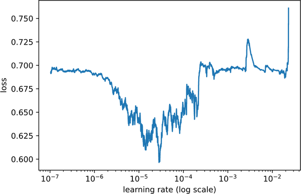
Figure 4-1. Finding a good learning rate using the visual plot of loss versus learning rate (log scale)

Using the output from lr_find(), and visually inspecting the loss plot as shown in Figure 4-1, you can start training the model using a learning rate, which has the least loss. This will enable you to get to a good start when training the model.

Using Hugging Face and Transformers

In the previous section, we showed how you can use ktrain to perform text classification. As you get familiar with using transformer-based models, you might want to leverage the full capabilities of the Hugging Face Python library directly.

In this section, we show you how you can use Hugging Face and one of the state-of-the-art transformers in Hugging Face called RoBERTa. RoBERTa uses an architecture similar to BERT and uses a byte-level BPE as a tokenizer. RoBERTa made several other optimizations to improve the BERT architecture. These include bigger batch size, longer training time, and using more diversified training data.

Loading the Relevant Python Packages

Let’s start by loading the relevant Hugging Face Transformer libraries and sklearn.

In the code snippet, you will observe that we are loading several libraries. For example, we will be using RobertaForSequenceClassification and RobertaTokenizer for performing text classification and tokenization, respectively:

import numpy as np
import pandas as pd

from sklearn.preprocessing import LabelEncoder
from sklearn.linear_model import LogisticRegression
from sklearn.model_selection import cross_val_score
from sklearn.model_selection import train_test_split

import torch
import torch.nn as nn
import transformers as tfs

from transformers import AdamW, BertConfig
from transformers import RobertaTokenizer, RobertaForSequenceClassification

Dataset Preparation

Similar to the earlier sections, we will load the FakeNewsNet dataset. After we have loaded the fakenews_df DataFrame, we will extract the relevant columns that we will use to fine-tune the RoBERTa model:

# Read the FakeNewsNet dataset and show the first few rows
fakenews_df = pd.read_csv('../data/fakenews_snorkel_labels.csv')

X = fakenews_df.loc[:,['statement', 'snorkel_labels']]

# remove rows with a -1 snorkel_labels value
X = X[X['snorkel_labels'] >= 0]

labels = X.snorkel_labels

Next, we will split the data in X into the training, validation, and testing datasets. The training and validation dataset will be used when we train the model and do a model evaluation. The training, validation, and testing datasets are assigned to variables X_train, X_val, and X_test, respectively:

# Split the data into train/test datasets
X_train, X_test, y_train, y_test =
        train_test_split(X['statement'],
                         X['snorkel_labels'],
                         test_size=0.20,
                         random_state=122520)


# withold test cases for testing
X_test, X_val, y_test, y_val =
        train_test_split(X_test, y_test,
                         test_size=0.30,
                         random_state=122420)

Checking Whether GPU Hardware Is Available

In this section, we provide sample code to determine the number of available GPUs that can be used for training. In addition, we also print out the type of GPU:

if torch.cuda.is_available():
    device = torch.device("cuda")
    print(f'GPU(s) available: {torch.cuda.device_count()} ')
    print('Device:', torch.cuda.get_device_name(0))

else:
    device = torch.device("cpu")
    print('No GPUs available. Default to use CPU')

For example, running the preceding code on an Azure Standard NC6_Promo (6 vcpus, 56 GiB memory) Virtual Machine (VM), the following output is printed. The output will differ depending on the NVidia GPUs that are available on the machine that you are using for training:

GPU(s) available: 1
Device: Tesla K80

Performing Tokenization

Let’s learn how you can perform tokenization using the RoBERTa tokenizer.

In the code shown, you will see that we first load the pretrained roberta-base model using RobertaForSequenceClassification.from_pretrained(…).

Next, we also loaded the pretrained tokenizer using RobertaTokenizer.from_pretrained(…):

model = RobertaForSequenceClassification.from_pretrained(
            'roberta-base',
            return_dict=True)

tokenizer = RobertaTokenizer.from_pretrained('roberta-base')

Next, you will use tokenizer() to prepare the training and validation data by performing tokenization, truncation, and padding of the data. The encoded training and validation data is stored in the variables tokenized_train and tokenized_validation, respectively.

We specify padding= max_length to control the padding that is used. In addition, we specify truncation=True to make sure we truncate the inputs to the maximum length specified:

max_length = 256

# Use the Tokenizer to tokenize and encode
tokenized_train = tokenizer(
    X_train.to_list(),
    padding='max_length',
    max_length = max_length,
    truncation=True,
    return_token_type_ids=False,
)

tokenized_validation = tokenizer(
    X_val.to_list(),
    padding='max_length',
    max_length = max_length,
    truncation=True,
    return_token_type_ids=False
)

Note

Hugging Face v3.x introduced new APIs for all tokenizers. See the documentation for how to migrate from v2.x to v3.x. In this chapter, we are using the new v3.x APIs for tokenization.

Next, we will convert the tokenized input_ids, attention mask, and labels into Tensors that we can use as inputs to training:

# Convert to Tensor
train_input_ids_tensor =
            torch.tensor(tokenized_train["input_ids"])

train_attention_mask_tensor =
            torch.tensor(tokenized_train["attention_mask"])

train_labels_tensor = torch.tensor(y_train.to_list())


val_input_ids_tensor =
          torch.tensor(tokenized_validation ["input_ids"])

val_attention_mask_tensor =
          torch.tensor(tokenized_validation ["attention_mask"])

val_labels_tensor = torch.tensor(y_val.to_list())

Model Training

Before we start to fine-tune the RoBERTa model, we’ll create the DataLoader for both the training and validation data. The DataLoader will be used during the fine-tuning of the model. To do this, we first convert the inputs_ids, attention_mask, and labels to a TensorDataset. Next, we create the DataLoader using the TensorDataset as inputs and specify the batch size. We set the variable batch_size to be 16:

# Preparing the DataLaoders
from torch.utils.data import TensorDataset, DataLoader
from torch.utils.data import RandomSampler

# Specify a batch size of 16
batch_size = 16

# 1. Create a TensorDataset
# 2. Define the data sampling approach
# 3. Create the DataLoader
train_data_tensor = TensorDataset(train_input_ids_tensor,
             train_attention_mask_tensor,
             train_labels_tensor)

train_dataloader = DataLoader(train_data_tensor,
             batch_size=batch_size,
             shuffle=True)

val_data_tensor = TensorDataset(val_input_ids_tensor,
             val_attention_mask_tensor,
             val_labels_tensor)

val_dataloader = DataLoader(val_data_tensor,
             batch_size=batch_size,
             shuffle=True)

Next, we specify the number of epochs that will be used for fine-tuning the model and also compute the total_steps needed based on the number of epochs, and the number of batches in train_dataloader:

num_epocs = 2
total_steps = num_epocs * len(train_dataloader)

Next, we specify the optimizer that will be used. For this exercise, we will use the AdamW optimizer, which is part of the Hugging Face optimization module. The AdamW optimizer implements the Adam algorithm with the weight decay fix that can be used when fine-tuning models.

In addition, you will notice that we specified a scheduler, using get_linear_schedule_with_warmup(). This creates a schedule with a learning rate that decreases linearly, using the initial learning rate that was set in the optimizer as the reference point. The learning rate decreases linearly after a warm-up period:

# Use the Hugging Face optimizer
from transformers import AdamW
from transformers import get_linear_schedule_with_warmup


optimizer = AdamW(model.parameters(), lr = 3e-5)

# Create the learning rate scheduler.
scheduler = get_linear_schedule_with_warmup(optimizer,
           num_warmup_steps = 100,
           num_training_steps = total_steps)

Note

The Hugging Face optimization module provides several optimizers, learning schedulers, and gradient accumulators. See this site for how to use the different capabilities provided by the Hugging Face optimization module.

Now that we have the optimizer and scheduler created, we are ready to define the fine-tuning training function called train(). First, we set the model to be in training mode. Next, we iterate through each batch of data that is obtained from the train_dataloader. We use optimizer.zero_grad() to clear previously calculated gradients. Next, we invoke the forward pass with the model() function and retrieve both the loss and logits after it completes. We add the loss obtained to the total_loss and then invoke the backward pass by calling loss.backward().

To mitigate the exploding gradient problem, we clip the normalized gradiated to 1.0. Next, we update the parameters using optimizer.step():

def train():
  total_loss = 0.0
  total_preds=[]

  # Set model to training mode
  model.train()

  # Iterate over the batch in dataloader
  for step,batch in enumerate(train_dataloader):
    # Get it batch to leverage device
    batch = [r.to(device) for r in batch]
    input_ids, mask, labels = batch

    model.zero_grad()
    outputs = model(input_ids,attention_mask=mask, labels=labels)

    loss = outputs.loss
    logits = outputs.logits

    # add on to the total loss
    total_loss = total_loss + loss

    # backward pass
    loss.backward()

    # Reduce the effects of the exploding gradient problem
    torch.nn.utils.clip_grad_norm_(model.parameters(), 1.0)

    # update parameters
    optimizer.step()

    # Update the learning rate.
    scheduler.step()

    # append the model predictions
    total_preds.append(outputs)

  # compute the training loss of the epoch
  avg_loss = total_loss / len(train_dataloader)



  #returns the loss and predictions
  return avg_loss

Similar to how we defined the fine-tuning function, we define the evaluation function, which is called evaluate(). We set the model to be in the evaluation model and iterate through each batch of data provided by val_dataloader. We used torch.no_grad() as we do not require the gradients during the evaluation of the model.

The average validation loss is computed once we have iterated through all the batches of validation data:

def evaluate():
  total_loss = 0.0
  total_preds = []

  # Set model to evaluation mode
  model.eval()

  # iterate over batches
  for step,batch in enumerate(val_dataloader):
    batch = [t.to(device) for t in batch]
    input_ids, mask, labels = batch

    # deactivate autograd
    with torch.no_grad():
      outputs = model(input_ids,attention_mask=mask, labels=labels)

      loss = outputs.loss
      logits = outputs.logits

      # add on to the total loss
      total_loss = total_loss + loss
      total_preds.append(outputs)

  # compute the validation loss of the epoch
  avg_loss = total_loss / len(val_dataloader)

  return avg_loss

Now that we have defined both the training and evaluation function, we are ready to start fine-tuning the model and performing an evaluation.

We first push the model to the available GPU and then iterate through multiple epochs. For each epoch, we invoke the train() and evaluate() functions and obtain both the training and validation loss.

Whenever we find a better validation loss, we will save the model to disk by invoking torch.save() and update the variable best_val_loss:

train_losses=[]
valid_losses=[]

# set initial loss to infinite
best_val_loss = float('inf')

# push the model to GPU
model = model.to(device)

# Specify the name of the saved weights file
saved_file = "fakenewsnlp-saved_weights.pt"

# for each epoch
for epoch in range(num_epocs):
    print('\n Epoch {:} / {:}'.format(epoch + 1, num_epocs))

    train_loss = train()
    val_loss = evaluate()

    print(f' Loss: {train_loss:.3f} - Val_Loss: {val_loss:.3f}')

    # save the best model
    if val_loss < best_val_loss:
        best_val_loss = val_loss
        torch.save(model.state_dict(),  saved_file)

    # Track the training/validation loss
    train_losses.append(train_loss)
    valid_losses.append(val_loss)

# Release the memory in GPU
model.cpu()
torch.cuda.empty_cache()

When we run the code, you will see the output with the training and validation loss for each epoch. In this example, the output terminates at epoch 2, and we have now a fine-tuned RoBERTa model using the data from the FakeNewsNet dataset:

Epoch 1 / 2
Loss: 0.649 - Val_Loss: 0.580

Epoch 2 / 2
Loss: 0.553 - Val_Loss: 0.546

Testing the Fine-Tuned Model

Let’s run the fine-tuned RoBERTa model on the test dataset. Similar to how we prepared the training and validation datasets earlier, we will start by tokenizing the test data, performing truncation, and padding:

tokenized_test = tokenizer(
    X_test.to_list(),
    padding='max_length',
    max_length = max_length,
    truncation=True,
    return_token_type_ids=False
)

Next, we prepare the test_dataloader that we will use for testing:

test_input_ids_tensor = torch.tensor(tokenized_test["input_ids"])
test_attention_mask_tensor = torch.tensor(tokenized_test["attention_mask"])
test_labels_tensor = torch.tensor(y_test.to_list())

test_data_tensor = TensorDataset(test_input_ids_tensor,
                               test_attention_mask_tensor,
                               test_labels_tensor)

test_dataloader = DataLoader(test_data_tensor,
                             batch_size=batch_size,
                             shuffle=False)

We are now ready to test the fine-tuned RoBERTa model. To do this, we iterate through multiple batches of data provided by test_dataloader. To obtain the predicted label, we use torch.argmax() to get the label using the logits that are provided. The predicted results are then stored in the variable predictions:

total_preds = []
predictions = []

model = model.to(device)

# Set model to evaluation mode
model.eval()

# iterate over batches
for step,batch in enumerate(test_dataloader):
   batch = [t.to(device) for t in batch]
   input_ids, mask, labels = batch

   # deactivate autograd
   with torch.no_grad():
      outputs = model(input_ids,attention_mask=mask)
      logits = outputs.logits

      predictions.append(torch.argmax(logits, dim=1).tolist())
      total_preds.append(outputs)


model.cpu()

Now that we have the predicted results, we are ready to compute the performance metrics of the model. We will use sklearn classification report to get the different performance metrics for the evaluation:

from sklearn.metrics import classification_report

y_true = y_test.tolist()
y_pred =  list(np.concatenate(predictions).flat)
print(classification_report(y_true, y_pred))

The output of running the code is shown:

              precision    recall  f1-score   support

           0       0.76      0.52      0.62       816
           1       0.66      0.85      0.74       885

    accuracy                           0.69      1701
   macro avg       0.71      0.69      0.68      1701
weighted avg       0.71      0.69      0.68      1701

Summary

Snorkel has been used in many real-world NLP applications across industry, medicine, and academia. At the same time, the field of NLP is evolving at a rapid pace. Transformer-based models have enabled many NLP tasks to be performed with high-quality results.

In this chapter, you learned how to use Hugging Face and ktrain to perform text classification for a FakeNewsNet dataset, which has been labeled by Snorkel in Chapter 3.

By combining the power of Snorkel for weak labeling and NLP libraries like Hugging Face, ML practitioners can get started with developing innovative NLP applications!

¹ Sebastian Ruder et al., “Transfer Learning in Natural Language Processing,” Slide presentation, Conference of the North American Chapter of the Association for Computational Linguistics [NAACL-HLT], Minneapolis, MN, June 2, 2019, https://oreil.ly/5hyM8.

² Anna Rogers, Olga Kovaleva, and Anna Rumshisky, “A Primer in BERTology: What We Know About How BERT Works” (Preprint, submitted November 9, 2020), https://arxiv.org/abs/2002.12327.

³ Peter Bloem, “Transformers from Scratch,” Peter Bloem (blog), video lecture, August 18, 2019, http://peterbloem.nl/blog/transformers.

⁴ Jay Alammar, “The Illustrated Transformer,” jalammar.github (blog), June 27, 2018, http://jalammar.github.io/illustrated-transformer.

⁵ Jakob Uszkoreit, “Transformer: A Novel Neural Network Architecture for Language Understanding,” Google AI Blog, August 31, 2017, https://ai.googleblog.com/2017/08/transformer-novel-neural-network.html.

⁶ Victor Sanh et al., “DistilBERT, A Distilled Version of BERT: Smaller, Faster, Cheaper and Lighter” (Preprint, submitted March 1, 2020), https://arxiv.org/abs/1910.01108.

⁷ Alec Radford et al., “Improving Language Understanding by Generative Pre-Training” (Preprint, submitted 2018), OpenAI, University of British Columbia, accessed August 13, 2021, https://www.cs.ubc.ca/~amuham01/LING530/papers/radford2018improving.pdf.