Predictive Control of Power Converters and Electrical Drives

4.7 Working Principle

In order to illustrate how the predictive control strategy works, a detailed example is shown in Figure 4.5 and Figure 4.6. Here, load currents i_α, i_β, and their references are shown for a complete period of the reference. Using the measurement i(k) and all switching states of the voltage vector v(k), the future currents i(k + 1) are estimated, i^p(k + 1).

Figure 4.4 Voltage vectors in the complex plane

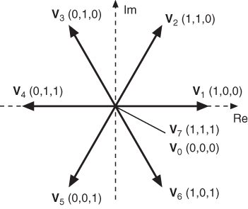
Figure 4.5 Working principle: vectorial plot of the reference and predicted currents

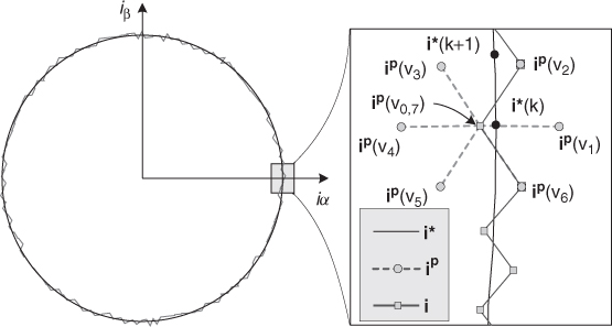
In the vectorial plot, shown in Figure 4.5, it can be observed that vector V₂ takes the predicted current vector closest to the reference vector.

As shown in Figure 4.6, current corresponds to the predicted current if the voltage vector V₀ or V₇ is applied at time k. It can be seen in this figure that vectors V₂ and V₆ are the ones that minimize the error in the i_α current, and vectors V₂ and V₃ are the ones that minimize the error in the i_β current, so the voltage vector that minimizes the cost function g is V₂.

These figures illustrate the meaning of the cost function as a measure of error or distance between reference and predicted vectors. It is easy to view these errors ...