Quantitative Finance for Physicists

10.2 CAPITAL ASSET PRICING MODEL (CAPM)

The Capital Asset Pricing Model (CAPM) is based on the portfolio

selection approach outlined in the previous section. Let us consider

the entire universe of risky assets with all possible returns and risks.

The set of optimal portfolios in this universe (i.e., portfolios with

maximal returns for given risks) forms what is called a efficient

frontier. The straight line that is tangent to the efficient frontier and

has intercept R

f

is called the capital market line.

2

The tangency point

between the capital market line and the efficient frontier corresponds

to the so-called super-efficient portfolio.

In CAPM, it is assumed that all investors have homogenous expect-

ations of returns, risks, and correlations among the risky assets. It is

also assumed that investors behave rationally, meaning they all hold

optimal mean-variance efficient portfolios. This implies that all invest-

ors have risky assets in their portfolio in the same proportions as the

entire market. Hence, CAPM promotes passive investing in the index

0

0.04

0.08

0.12

0.16

0 0.04 0.08 0.12 0.16

sigma

E[R]

RF

T

P

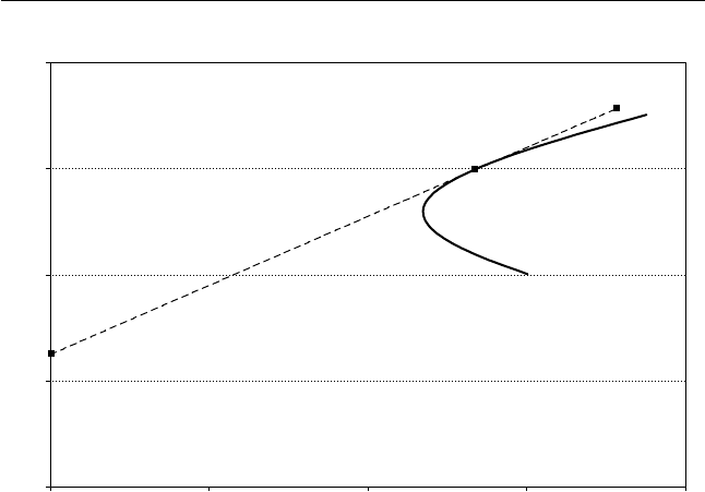
Figure 10.1 The return-risk trade-off lines: portfolio with the risk-free

asset and a risky asset (dashed line); portfolio with two risky assets (solid

line); R

f

¼ 0:05, s

1

¼ 0:12, s

2

¼ 0:15, E[R

1

] ¼ 0:08, E[R

2

] ¼ 0:14.

114 Portfolio Management

mutual funds. Within CAPM, the optimal investing strategy is simply

choosing a portfolio on the capital market line with acceptable risk

level. Therefore, the difference among rational investors is determined

only by their risk aversion, which is characterized with the proportion

of their wealth allocated to the risk-free assets. Within the CAPM

assumptions, it can be shown that the super-efficient portfolio consists

of all risky assets weighed with their market values. Such a portfolio is

called a market portfolio.

3

CAPM defines the return of a risky asset i with the security market

line

E[R

i

] ¼ R

f

þ b

i

(E[R

M

]  R

f

) (10:2:1)

where R

M

is the market portfolio return and parameter beta b

i

equals

b

i

¼ Cov[R

i

,R

M

]=Var[R

M

] (10:2:2)

Beta defines sensitivity of the risky asset i to the market dynamics.

Namely, b

i

> 1 means that the asset is more volatile than the entire

market while b

i

< 1 implies that the asset has a lower sensitivity to the

market movements. The excess return of asset i per unit of risk (so-

called Sharpe ratio) is another criterion widely used for estimation of

investment performance

S

i

¼ (E[R

i

]  R

f

)=s

i

(10:2:3)

CAPM, being the equilibrium model, has no time dependence. How-

ever, econometric analysis based on this model can be conducted

providing that the statistical nature of returns is known [2]. It is

often assumed that returns are independently and identically distrib-

uted. Then the OLS method can be used for estimating b

i

in the

regression equation for the excess return Z

i

¼ R

i

 R

f

Z

i

(t) ¼ a

i

þ b

i

Z

M

(t) þ e

i

(t) (10:2:4)

It is usually assumed that e

i

(t) is a normal process and the S&P 500

Index is the benchmark for the market portfolio return R

M

(t). More

details on the CAPM validation and the general results for the mean-

variance efficient portfolios can be found in [2, 3].

As indicated above, CAPM is based on the belief that investing in

risky assets yields average returns higher than the risk-free return.

Hence, the rationale for investing in risky assets becomes question-

able in bear markets. Another problem is that the asset diversification

Portfolio Management 115