Quantitative Finance for Physicists

Chapter 11

Market Risk Measurement

The widely used risk measure, value at risk (VaR), is discussed in

Section 11.1. Furthermore, the notion of the coherent risk measure is

introduced and one such popular measure, namely expected tail losses

(ETL), is described. In Section 11.2, various approaches to calculating

risk measures are discussed.

11.1 RISK MEASURES

There are several possible causes of financial losses. First, there is

market risk that results from unexpected changes in the market prices,

interest rates, or foreign exchange rates. Other types of risk relevant

to financial risk management include liquidity risk, credit risk, and

operational risk [1]. The liquidity risk closely related to market risk is

determined by a finite number of assets available at a given price (see

discussion in Section 2.1). Another form of liquidity risk (so-called

cash-flow risk) refers to the inability to pay off a debt in time. Credit

risk arises when one of the counterparts involved in a financial

transaction does not fulfill its obligation. Finally, operational risk is

a generic notion for unforeseen human and technical problems, such

as fraud, accidents, and so on. Here we shall focus exclusively on

measurement of the market risk.

In Chapter 10, we discussed risk measures such as the asset return

variance and the CAPM beta. Several risk factors used in APT were

121

also mentioned. At present, arguably the most widely used risk meas-

ure is value at risk (VaR) [1]. In short, VaR refers to the maximum

amount of an asset that is likely to be lost over a given period at a

specific confidence level. This implies that the probability density

function for profits and losses (P=L)

1

is known. In the simplest case,

this distribution is normal

P

N

(x) ¼

1

ffiffiffiffiffiffi

2p

p

s

exp [(x  m)

2

=2s

2

] (11:1:1)

where m and s are the mean and standard deviation, respectively.

Then for the chosen confidence level a,

VAR(a) ¼sz

a

 m (11:1:2)

The value of z

a

can be determined from the cumulative distribution

function for the standard normal distribution (3.2.10)

Pr(Z < z

a

) ¼

ð

z

a

1

1

ffiffiffiffiffiffi

2p

p

exp [z

2

=2]dz ¼ 1  a (11 :1 :3)

Since z

a

< 0ata > 50%, the definition (11.1.2) implies that positive

values of VaR point to losses. In general, VaR(a) grows with the

confidence level a. Sufficiently high values of the mean

P=L(m > sz

a

) for given a move VaR(a) into the negative region,

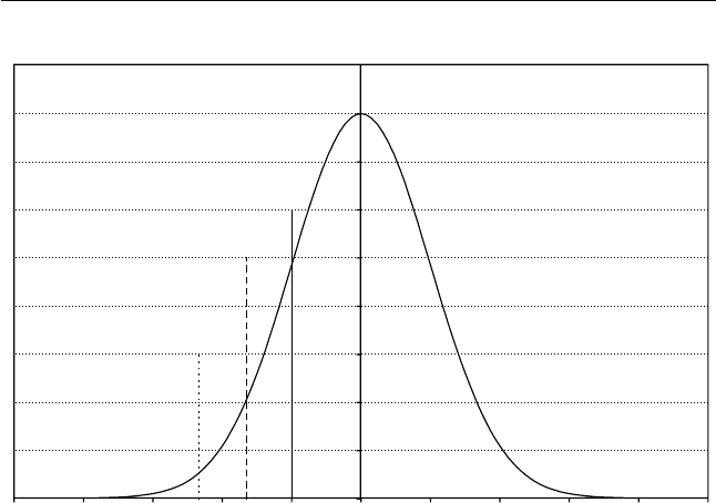
which implies profits rather than losses. Examples of z

a

for typical

values of a ¼ 95% and a ¼ 99% are given in Figure 11.1. Note that

the return variance s corresponds to z

a

¼1 and yields a  84%.

The advantages of VaR are well known. VaR is a simple and

universal measure that can be used for determining risks of different

financial assets and entire portfolios. Still, VaR has some drawbacks

[2]. First, accuracy of VaR is determined by the model assumptions

and is rather sensitive to implementation. Also, VaR provides an

estimate for losses within a given confidence interval a but says

nothing about possible outcomes outside this interval. A somewhat

paradoxical feature of VaR is that it can discourage investment

diversification. Indeed, adding volatile assets to a portfolio may

move VaR above the chosen risk threshold. Another problem with

VaR is that it can violate the sub-additivity rule for portfolio risk.

According to this rule, the risk measure r must satisfy the condition

122 Market Risk Measurement

r(A þ B)  r(A) þ r(B) (11:1:4)

which means the risk of owning the sum of two assets must not be

higher than the sum of the individual risks of these assets. The

condition (11.1.4) immediately yields an upper estimate of combined

risk. Violation of the sub-additivity rule may lead to several problems.

In particular, it may provoke investors to establish separate accounts

for every asset they have. Unfortunately, VaR satisfies (11.1.4) only if

the probability density function for P/L is normal (or, more generally,

elliptical) [3].

The generic criterions for the risk measures that satisfy the require-

ments of the modern risk management are formulated in [3]. Besides

the sub-additivity rule (11.1.4), they include the following conditions.

r(lA) ¼ lr(A), l > 0 (homogeneity) (11:1:5)

r(A)  r(B), if A  B (monotonicity) (11:1:6)

r(A þ C) ¼ r(A)  C (translation invariance) (11:1:7)

In (11.1.7), C represents a risk-free amount. Adding this amount to

a risky portfolio should decrease the total risk, since this amount is

0

0.05

0.1

0.15

0.2

0.25

0.3

0.35

0.4

0.45

−5 −4 −3 −2 −1012345

VaR at 95%

z = −1.64

VaR at 99%

z = −2.33

VaR at 84%

z = −1

Figure 11.1 VaR for the standard normal probability distribution of P/L.

Market Risk Measurement 123