model [11] was modified to describe the arrival of news in the market,
which affects the fundamental price. This process was modeled with
the Gaussian random variable e(t) so that
ln P
f
(t) ln P
f
(t 1) ¼ e(t) (12:3:9)
The modeling results exhibited the power-law scaling and temporal
volatility dependence in the price distributions.
12.4 THE OBSERVABLE VARIABLES MODEL
12.4.1 T
HE FRAMEWORK
The models discussed so far are capable of reproducing important
features of financial market dynamics. Yet, one may notice a degree
of arbitrariness in this field. The number of different agent types and
the rules of their transition and adaptation vary from one model to
another. Also, little is known about optimal choice of the model
parameters [15, 16]. As a result, many interesting properties, such as
deterministic chaos, may be the model artifacts rather than reflections
of the real world.
5
A parsimonious approach to choosing variables in the agent-based
modeling of financial markets was offered in [17]. Namely, it was
suggested to derive agent-based models exclusively in terms of observ-
able variables. Note that the notion of observable data in finance
should be discerned from the notion of publicly available data. While
the transaction prices in regulated markets are publicly available, the
market microstructure is not (see Section 2.1). Still, every event in the
financial markets that affects the market microstructure (such as
quote submission, quote cancellation, transactions, etc.) is recorded
and stored for business and legal purposes. This information allows
one to reconstruct the market microstructure at every moment. We
define observable variables in finance as those that can be retrieved or
calculated from the records of market events. Whether these records
are publicly available at present is a secondary issue. More import-
antly, these data exist and can therefore potentially be used for
calibrating and testing the theoretical models.
The numbers of agents of different types generally are not observ-
able. Indeed, consider a market analog of ‘‘Maxwell’s Demon’’ who is
136 Agent-Based Modeling of Financial Markets
able to instantly parse all market events. The Demon cannot discern
‘‘chartists’’ and ‘‘fundamentalists’’ in typical situations, such as when
the current price, being lower than the fundamental price, is growing.
In this case, all traders buy rather than sell. Similarly, when the
current price, being higher than the fundamental price, is falling, all
traders sell rather than buy.
Only price, the total number of buyers, and the total number of
sellers are always observable. Whether a trader becomes a buyer or
seller can be defined by mixing different behavior patterns in the
trader decision-making rule. Let us describe a simple non-equilibrium
price model derived along these lines [17]. We discern ‘‘buyers’’ (þ)
and ‘‘sellers’’ (). Total number of traders is N
N
þ
(t) þ N
(t) ¼ N (12:4:1)
The scaled numbers of buyers, n
þ
(t) ¼ N
þ
(t)=N, and sellers, n
(t)
¼ N
(t)=N, are described with equations
dn
þ
=dt ¼ v
þ
n
v
þ
n
þ
(12:4:2)
dn
=dt ¼ v
þ
n
þ
v
þ
n
(12:4:3)
The factors v
þ
and v
þ
characterize the probabilities for transfer
from seller to buyer and back, respectively
v
þ
¼ 1=v
þ
¼ n exp (U), U ¼ ap
1
dp=dt þ b(1 p) (12:4:4)
Price p(t) is given in units of its fundamental value. The first term in
the utility function, U, characterizes the ‘‘chartist’’ behavior while the
second term describes the ‘‘fundamentalist’’ pattern. The factor n has
the sense of the frequency of transitions between seller and buyer
behavior. Since n
þ
(t) ¼ 1 n
(t), the system (12.4.1)–(12.4.3) is re-
duced to the equation
dn
þ
=dt ¼ v
þ
(1 n
þ
) v
þ
n
þ
(12:4:5)
The price formation equation is assumed to have the following
form
dp=dt ¼ gD
ex
(12:4:6)
where the excess demand, D
ex
, is proportional to the excess number of
buyers
D
ex
¼ d(n
þ
n
) ¼ d(2n
þ
1) (12:4:7)
Agent-Based Modeling of Financial Markets 137
12.4.2 PRICE-DEMAND RELATIONS
The model described above is defined with two observable vari-
ables, n
þ
(t) and p(t). In equilibrium, its solution is n
þ
¼ 0:5 and
p ¼ 1. The necessary stability condition for this model is
adgn 1 (12:4:8)
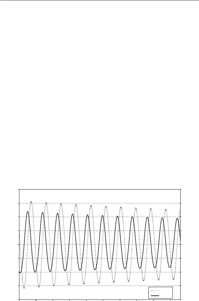
The typical stable solution for this model (relaxation of the initially
perturbed values of n
þ
and p) is given in Figure 12.1. Lower values of
a and g suppress oscillations and facilitate relaxation of the initial
perturbations. Thus, the rise of the ‘‘chartist’’ component in the utility
function increases the price volatility. Numerical solutions with the
values of a and g that slightly violate the condition (12.4.8) can lead to
the limit cycle providing that the initial conditions are very close to
the equilibrium values (see Figure 12.2). Otherwise, violation of the
condition (12.4.8) leads to system instability, which can be interpreted
as a market crash.
The basic model (12.4.1)–(12.4.7) can be extended in several
ways. First, the condition of the constant number of traders (12.4.1)
0.8
0.85
0.9
0.95
1
1.05
1.1
1.15
1.2
0 5 10 15 20 25 30 35 40 45
Time
Price
−0.4
−0.3
−0.2
−0.1
0
0.1
0.2
0.3
0.4
Dex
Price
Dex
Figure 12.1 Dynamics of excess demand (Dex) and price for the model
(12.4.5)–(12.4.7) with a ¼ b ¼ g ¼ 1, n
þ
(0) ¼ 0.4 and p(0) ¼ 1.05.
138 Agent-Based Modeling of Financial Markets
Get Quantitative Finance for Physicists now with the O’Reilly learning platform.
O’Reilly members experience books, live events, courses curated by job role, and more from O’Reilly and nearly 200 top publishers.

