The following steps decompose the time series:
- Read the data. The file has the Bureau of Labor Statistics monthly price data for unleaded gas and white flour for 1980 through 2014:
> prices <- read.csv("prices.csv")
- Create and plot the time series of gas prices:
prices.ts = ts(prices, start = c(1980,1), frequency = 12)
> plot(prices.ts)
The following is the plot of time versus prices as per our command:
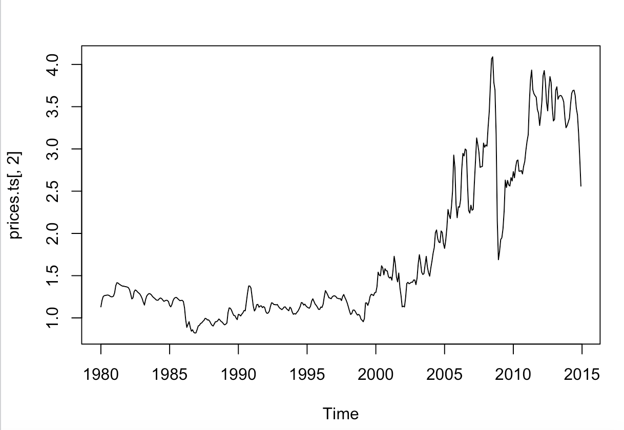
- The preceding plot shows seasonality in gas prices. The amplitude of fluctuations seems to increase with time, and hence this looks like a multiplicative time series. Thus, we will use the log of the prices to make it ...

