Statistics: An Introduction Using R, 2nd Edition

3Central Tendency

Despite the fact that everything varies, measurements often cluster around certain intermediate values; this attribute is called central tendency. Even if the data themselves do not show much tendency to cluster round some central value, the parameters derived from repeated experiments (e.g. replicated sample means) almost inevitably do (this is called the central limit theorem; see p. 70). We need some data to work with. The data are in a vector called y stored in a text file called yvalues

yvals <- read.csv("c:\\temp\\yvalues.csv")
attach(yvals)

So how should we quantify central tendency? Perhaps the most obvious way is just by looking at the data, without doing any calculations at all. The data values that occur most frequently are called the mode, and we discover the value of the mode simply by drawing a histogram of the data like this:

hist(y)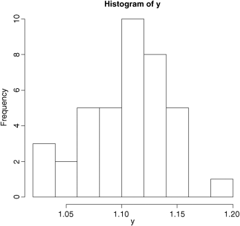

So we would say that the modal class of y was between 1.10 and 1.12 (we will see how to control the location of the break points in a histogram later).

The most straightforward quantitative measure of central tendency is the arithmetic mean of the data. This is the sum of all the data values divided by the number of data values, n. The capital Greek sigma just means ‘add up all the values’ of what follows; in this ...