Student Solutions Manual to Accompany Loss Models: From Data to Decisions, Fourth Edition

CHAPTER 4

CHAPTER 4 SOLUTIONS

4.1   SECTION 4.2

4.1 Arguing as in the examples,

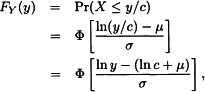
which indicates that Y has the lognormal distribution with parameters μ + ln c and σ. Because no parameter was multiplied by c, there is no scale parameter. To introduce a scale parameter, define the lognormal distribution function as . Note that the new parameter v is simply e^μ. Then, arguing as before,

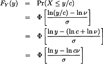
demonstrating that v is a scale parameter.

4.2 The following is not the only possible set of answers to this question. Model 1 is a uniform distribution on the interval 0 to 100 with parameters 0 and 100. It is also a beta distribution with parameters a = 1, b = 1, and θ = 100. Model 2 is a Pareto distribution with parameters α = 3 and θ = 2000. Model 3 would not normally be considered a parametric distribution. However, we could define a parametric discrete distribution with arbitrary probabilities at 0, 1, 2, 3, and 4 being the parameters. Conventional usage would not accept this as a parametric distribution. Similarly, Model 4 is not a standard parametric distribution, but we could define one as having arbitrary probability p at zero and an exponential distribution elsewhere. Model 5 could be from ...