Chapter 4. Reusable Model Elements
Developing an ML model can be a daunting task. Besides the data engineering aspect of the task, you also need to understand how to build the model. In the early days of ML, tree-based models (such as random forests) were king for applying straight-up classification or regression tasks to tabular datasets, and model architecture was determined by parameters related to model initialization. These parameters, known as hyperparameters, include the number of decision trees in a forest and the number of features considered by each tree when splitting a node. However, it is not straightforward to convert some types of data, such as images or text, into tabular form: images may have different dimensions, and texts vary in length. That’s why deep learning has become the de facto standard model architecture for image and text classification.
As deep-learning architecture gains popularity, a community has grown around it. Creators have built and tested different model structures for academic and Kaggle challenges. Many have made their models open source so that they are available for transfer learning—anyone can use them for their own purposes.
For example, ResNet is an image classification model trained on the ImageNet dataset, which is about 150GB in size and contains more than a million images. The labels in this data include plants, geological formations, natural objects, sports, persons, and animals. So how can you reuse the ResNet model to classify your own set of images, even with different categories or labels?
Open source models such as ResNet have very complicated structures. While the source code is available for anyone to access on sites like GitHub, downloading the source code is not the most user-friendly way to reproduce or reuse these models. There are almost always other dependencies that you have to overcome to compile or run the source code. So how can we make such models available and usable to nonexperts?
TensorFlow Hub (TFH) is designed to solve this problem. It enables transfer learning by making a variety of ML models freely available as libraries or web API calls. Anyone can write just a single line of code to load the model. All models can be invoked via a simple web call, and then the entire model is downloaded to your source code’s runtime. You don’t need to build the model yourself.
This definitely saves development and training time and increases accessibility. It also allows users to try out different models and build their own applications more quickly. Another benefit of transfer learning is that since you are not retraining the whole model from scratch, you may not need a high-powered GPU or TPU to get started.
In this chapter, we are going to take a look at just how easy it is to leverage TensorFlow Hub. So let’s start with how TFH is organized. Then you’ll download one of the TFH pretrained image classification models and see how to use it for your own images.
The Basic TensorFlow Hub Workflow
TensorFlow Hub (Figure 4-1) is a repository of pretrained models curated by Google. Users may download any model into their own runtime and perform fine-tuning and training with their own data.
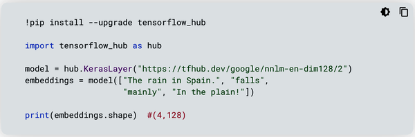
Figure 4-1. TensorFlow Hub home page
To use TFH, you must install it via the familiar Pythonic pip install command in your Python cell or terminal:
pip install --upgrade tensorflow_hub
Then you can start using it in your source code by importing it:
import tensorflow_hub as hub
First, invoke the model:
model = hub.KerasLayer("https://tfhub.dev/google/nnlm-en-dim128/2")
This is a pretrained text embedding model. Text embedding is the process of mapping a string of text to a multidimensional vector of numeric representation. You can give this model four text strings:
embeddings = model(["The rain in Spain.", "falls",
                      "mainly", "In the plain!"])
Before you look at the results, inspect the shape of the model output:
print(embeddings.shape)
It should be:
(4, 128)
There are four outputs, each 128 units long. Figure 4-2 shows one of the outputs:
print(embeddings[0])
Figure 4-2. Text embedding output
As indicated in this simple example, you did not train this model. You only loaded it and used it to get a result with your own data. This pretrained model simply converts each text string into a vector representation of 128 dimensions.
On the TensorFlow Hub home page, click the Models tab. As you can see, TensorFlow Hub categorizes its pretrained models into four problem domains: image, text, video, and audio.
Figure 4-3 shows the general pattern for a transfer learning model.
From Figure 4-3, you can see that the pretrained model (from TensorFlow Hub) is sandwiched between an input layer and an output layer, and there can be some optional layers prior to the output layer.
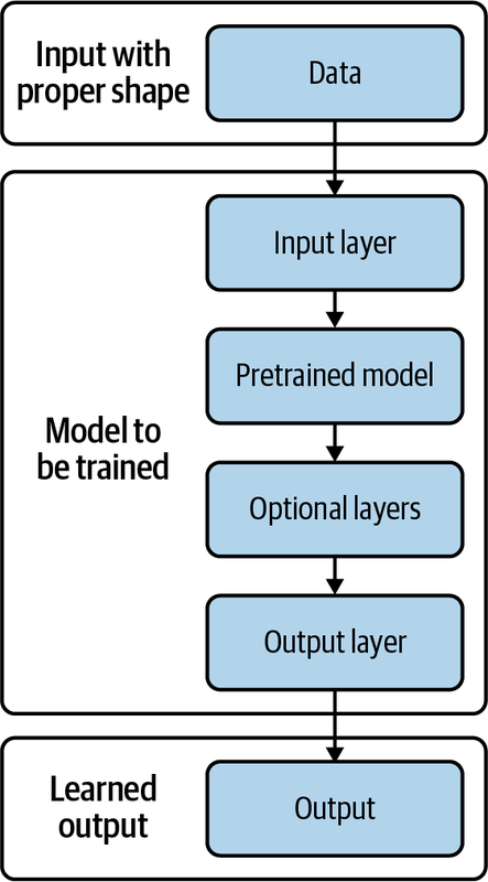
Figure 4-3. General pattern for transfer learning
To use any of the models, you’ll need to address a few important considerations, such as input and output:
- Input layer
-
Input data must be properly formatted (or “shaped”), so pay special attention to each model’s input requirements (found in the Usage section on the web page that describes the individual model). Take the ResNet feature vector, for example: the Usage section states the required size and color values for the input images and that the output is a batch of feature vectors. If your data does not meet the requirements, you’ll need to apply some of the data transformation techniques you learned in “Preparing Image Data for Processing”.
- Output layer
-
Another important and necessary element is the output layer. This is a must if you wish to retrain the model with your own data. In the simple embedding example shown earlier, we didn’t retrain the model; we merely fed it a few text strings to see the model output. An output layer serves the purpose of mapping the model output to the most likely labels if the problem is a classification problem. If it is a regression problem, then it serves to map the model output to a numeric value. A typical output layer is called “dense,” with either one node (for regression or binary classification) or multiple nodes (such as for multiclass classification).
- Optional layers
-
Optionally, you can add one or more layers before the output layer to improve model performance. These layers may help you extract more features to improve model accuracy, such as a convolution layer (Conv1D, Conv2D). They can also help prevent or reduce model overfitting. For example, dropout reduces overfitting by randomly setting an output to zero. If a node outputs an array such as [0.5, 0.1, 2.1, 0.9] and you set a dropout ratio of 0.25, then during training, by random chance, one of the four values in the array will be set to zero; for example, [0.5, 0, 2.1, 0.9]. Again, this is considered optional. Your training does not require it, but it may help improve your model’s accuracy.
Image Classification by Transfer Learning
We are going to walk through an image classification example with transfer learning. In this example, your image data consists of five classes of flowers. You will use the ResNet feature vector as your pretrained model. We will address these common tasks:
-
Model requirements
-
Data transformation and input processing
-
Model implementation with TFH
-
Output definition
-
Mapping output to plain-text format
Model Requirements
Let’s look at the ResNet v1_101 feature vector model. This web page contains an overview, a download URL, instructions, and, most importantly, the code you’ll need to use the model.
In the Usage section, you can see that to load the model, all you need to do is pass the URL to hub.KerasLayer. The Usage section also includes the model requirements. By default, it expects the input image, which is written as an array of shape [height, width, depth], to be [224, 224, 3]. The pixel value is expected to be within the range [0, 1]. As the output, it provides the Dense layer with the number of nodes, which reflects the number of classes in the training images.
Data Transformation and Input Processing
It is your job to transform your images into the required shape and normalize the pixel scale to within the required range. As we’ve seen, images usually come in different size and pixel values. A typical color JPEG image pixel value for each RGB channel might be anywhere from 0 to 225. So, we need operations to standardize image size to [224, 224, 3], and to normalize pixel value to a [0, 1] range. If we use ImageDataGenerator in TensorFlow, these operations are provided as input flags. Here’s how to load the images and create a generator:
Start by loading the libraries:
import tensorflow as tf
import tensorflow_hub as hub
import numpy as np
import matplotlib.pylab as plt
Load the data you need. For this example, let’s use the flower images provided by TensorFlow:
data_dir = tf.keras.utils.get_file(
    'flower_photos',
'https://storage.googleapis.com/download.tensorflow.org/
example_images/flower_photos.tgz',
    untar=True)
Open
data_dirand find the images. You can see the file structure in the file path:
!ls -lrt /root/.keras/datasets/flower_photos
Here is what will display:
total 620
-rw-r----- 1 270850 5000 418049 Feb  9  2016 LICENSE.txt
drwx------ 2 270850 5000  45056 Feb 10  2016 tulips
drwx------ 2 270850 5000  40960 Feb 10  2016 sunflowers
drwx------ 2 270850 5000  36864 Feb 10  2016 roses
drwx------ 2 270850 5000  53248 Feb 10  2016 dandelion
drwx------ 2 270850 5000  36864 Feb 10  2016 daisy
There are five classes of flowers. Each class corresponds to a directory.
Define some global variables to store pixel values and batch size (the number of samples in a batch of training images). You don’t yet need the third dimension of the image, just the height and width for now:
pixels =224
BATCH_SIZE = 32
IMAGE_SIZE = (pixels, pixels)
NUM_CLASSES = 5
Specify image normalization and a fraction of data for cross validation. It is a good idea to hold out a fraction of training data for cross validation, which is a means of evaluating the model training process through each epoch. At the end of each training epoch, the model contains a set of trained weights and biases. At this point, the data held out for cross validation, which the model has never seen, can be used as a test for model accuracy:
datagen_kwargs = dict(rescale=1./255, validation_split=.20)
dataflow_kwargs = dict(target_size=IMAGE_SIZE,
batch_size=BATCH_SIZE,
interpolation="bilinear")

valid_datagen = tf.keras.preprocessing.image.
ImageDataGenerator(
    **datagen_kwargs)
valid_generator = valid_datagen.flow_from_directory(
    data_dir, subset="validation", shuffle=False,
    **dataflow_kwargs)
The
ImageDataGeneratordefinition and generator instance both accept our arguments in a dictionary format. The rescaling factor and validation fraction go to the generator definition, while the standardized image size and batch size go to the generator instance.The
interpolationargument indicates that the generator needs to resample the image data totarget_size, which is 224 × 224 pixels.Now, do the same for the training data generator:
train_datagen = valid_datagen
train_generator = train_datagen.flow_from_directory(
    data_dir, subset="training", shuffle=True,
    **dataflow_kwargs)
Identify mapping of class index to class name. Since the flower classes are encoded in the index, you need a map to recover the flower class names:
labels_idx = (train_generator.class_indices)
idx_labels = dict((v,k) for k,v in labels_idx.items())
You can display the
idx_labelsto see how these classes are mapped:
idx_labels

{0: 'daisy', 1: 'dandelion', 2: 'roses', 3: 'sunflowers',
4: 'tulips'}
You’ve now normalized and standardized your image data. The image generators are defined and instantiated for training and validation data. You also have the label lookup to decode model prediction, and you’re ready to implement the model with TFH.
Model Implementation with TensorFlow Hub
As you saw back in Figure 4-3, the pretrained model is sandwiched between an input and an output layer. You can define this model structure accordingly:
model = tf.keras.Sequential([
     tf.keras.layers.InputLayer(input_shape=IMAGE_SIZE + (3,)),
hub.KerasLayer("https://tfhub.dev/google/imagenet/resnet_v1_101/
feature_vector/4", trainable=False),
     tf.keras.layers.Dense(NUM_CLASSES, activation='softmax',
name = 'flower_class')
])

model.build([None, 224, 224, 3]) !!C04!!
Notice a few things here:
-
There is an input layer that defines the input shape of images as [224, 224, 3].
-
When
InputLayeris invoked,trainableshould be set to False. This indicates that you want to reuse the current values from the pretrained model. -
There is an output layer called
Densethat provides the model output (this is described in the Usage section of the summary page).
After the model is built, you’re ready to start training. First, specify the loss function and pick an optimizer:
model.compile(
  optimizer=tf.keras.optimizers.SGD(lr=0.005, momentum=0.9),
loss=tf.keras.losses.CategoricalCrossentropy(
from_logits=True,
label_smoothing=0.1),
metrics=['accuracy'])
Then specify the number of batches for training data and cross-validation data:
steps_per_epoch = train_generator.samples //
train_generator.batch_size
validation_steps = valid_generator.samples //
valid_generator.batch_size
Then start the training process:
model.fit(
    train_generator,
    epochs=5, steps_per_epoch=steps_per_epoch,
    validation_data=valid_generator,
    validation_steps=validation_steps)
After the training process runs through all the epochs specified, the model is trained.
Defining the Output
According to the Usage guideline, the output layer Dense consists of a number of nodes, which reflects how many classes are in the expected images. This means each node outputs a probability for that class. It is your job to find which one of these probabilities is the highest and map that node to the flower class using idx_labels. Recall that the idx_labels dictionary looks like this:
{0: 'daisy', 1: 'dandelion', 2: 'roses', 3: 'sunflowers',
4: 'tulips'}
The Dense layer’s output consists of five nodes in the exact same order. You’ll need to write a few lines of code to map the position with the highest probability to the corresponding flower class.
Mapping Output to Plain-Text Format
Let’s use the validation images to understand a bit more about how to map the model prediction output to the actual class for each image. You’ll use the predict function to score these validation images. Retrieve the NumPy array for the first batch:
sample_test_images, ground_truth_labels = next(valid_generator)

prediction = model.predict(sample_test_images)
There are 731 images and 5 corresponding classes in the cross-validation data. Therefore, the output shape is [731, 5]:
array([[9.9994004e-01, 9.4704428e-06, 3.8405190e-10, 5.0486942e-05,
        1.0701914e-08],
       [5.9500107e-06, 3.1842374e-06, 3.5622744e-08, 9.9999082e-01,
        3.0683900e-08],
       [9.9994218e-01, 5.9974178e-07, 5.8693445e-10, 5.7049790e-05,
        9.6709634e-08],
       ...,
       [3.1268091e-06, 9.9986601e-01, 1.5343730e-06, 1.2935932e-04,
        2.7383029e-09],
       [4.8439368e-05, 1.9247003e-05, 1.8034354e-01, 1.6394027e-02,
        8.0319476e-01],
       [4.9799957e-07, 9.9232978e-01, 3.5823192e-08, 7.6697678e-03,
        1.7666844e-09]], dtype=float32)
Each row represents the probability distribution for the image class. For the first image, the highest probability, 1.0701914e-08 (highlighted in the preceding code), is in the last position, which corresponds to index 4 of that row (remember, the numbering of an index starts with 0).
Now you need to find the position where the highest probability occurs for each row, using this code:
predicted_idx = tf.math.argmax(prediction, axis = -1)
And if you display the results with the print command, you’ll see this:
print (predicted_idx)

<tf.Tensor: shape=(731,), dtype=int64, numpy=
array([0, 3, 0, 1, 0, 4, 4, 1, 2, 3, 4, 1, 4, 0, 4, 3, 1, 4, 4, 0,
       …
       3, 2, 1, 4, 1])>
Now, apply the lookup with idx_labels to each element in this array. For each element, use a function:
def find_label(idx):
    return idx_labels[idx]
To apply a function to each element of a NumPy array, you’ll need to vectorize the function:
find_label_batch = np.vectorize(find_label)
Then apply this vectorized function to each element in the array:
result = find_label_batch(predicted_idx)
Finally, output the result side by side with the image folder and filename so that you can save it for reporting or further investigation. You can do this with Python pandas DataFrame manipulation:
import pandas as pd
predicted_label = result_class.tolist()
file_name = valid_generator.filenames

results=pd.DataFrame({"File":file_name,
                      "Prediction":predicted_label})
Let’s take a look at the results dataframe, which is 731 rows × 2 columns.
| File | Prediction | |
|---|---|---|
| 0 | daisy/100080576_f52e8ee070_n.jpg | daisy |
| 1 | daisy/10140303196_b88d3d6cec.jpg | sunflowers |
| 2 | daisy/10172379554_b296050f82_n.jpg | daisy |
| 3 | daisy/10172567486_2748826a8b.jpg | dandelion |
| 4 | daisy/10172636503_21bededa75_n.jpg | daisy |
| ... | ... | ... |
| 726 | tulips/14068200854_5c13668df9_m.jpg | sunflowers |
| 727 | tulips/14068295074_cd8b85bffa.jpg | roses |
| 728 | tulips/14068348874_7b36c99f6a.jpg | dandelion |
| 729 | tulips/14068378204_7b26baa30d_n.jpg | tulips |
| 730 | tulips/14071516088_b526946e17_n.jpg | dandelion |
Evaluation: Creating a Confusion Matrix
A confusion matrix, which evaluates the classification results by comparing model output with ground truth, is the easiest way to get an initial feel for how well the model performs. Let’s look at how to create a confusion matrix.
You’ll use pandas Series as the data structure for building your confusion matrix:
y_actual = pd.Series(valid_generator.classes)
y_predicted = pd.Series(predicted_idx)
Then you’ll utilize pandas again to produce the matrix:
pd.crosstab(y_actual, y_predicted, rownames = ['Actual'],
colnames=['Predicted'], margins=True)
Figure 4-4 shows the confusion matrix. Each row represents the distribution of actual flower labels by predictions. For example, looking at the first row, you will notice that there are a total of 126 samples that are actually class 0, which is daisy. The model correctly predicted 118 of these images as class 0; four are misclassified as class 1, which is dandelion; one is misclassified as class 2, which is roses; three are misclassified as class 3, which is sunflowers; and none has been misclassified as class 4, which is tulips.
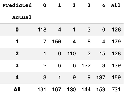
Figure 4-4. Confusion matrix for flower image classification
Next, use the sklearn library to provide a statistical report for each class of images:
from sklearn.metrics import classification_report
report = classification_report(truth, predicted_results)
print(report)
              precision    recall  f1-score   support

           0       0.90      0.94      0.92       126
           1       0.93      0.87      0.90       179
           2       0.85      0.86      0.85       128
           3       0.85      0.88      0.86       139
           4       0.86      0.86      0.86       159

    accuracy                           0.88       731
   macro avg       0.88      0.88      0.88       731
weighted avg       0.88      0.88      0.88       731
This result shows that the model has the best performance when classifying daisies (class 0), with an f1-score of 0.92. Its performance is worst in classifying roses (class 2), with an f1-score of 0.85. The “support” column indicates the sample size in each class.
Summary
You have just completed an example project using a pretrained model from TensorFlow Hub. You appended the necessary input layer, performed data normalization and standardization, trained the model, and scored a batch of images.
This experience shows the importance of meeting the model’s input and output requirements. Just as importantly, pay close attention to the output format of the pretrained model. (This information is all available in the model documentation page on the TensorFlow Hub website.) Finally, you also need to create a function that maps the model output to plain text to make it meaningful and interpretable.
Using the tf.keras.applications Module for Pretrained Models
Another place to find a pretrained model for your own use is the tf.keras.applications module (see the list of available models). When the Keras API became available in TensorFlow, this module became a part of the TensorFlow ecosystem.
Each model comes with pretrained weights, and using them is just as easy as using TensorFlow Hub. Keras provides the flexibility needed to conveniently fine-tune your models. By making each layer in a model accessible, tf.keras.applications lets you specify which layers to retrain and which layers to leave untouched.
Model Implementation with tf.keras.applications
As with TensorFlow Hub, you need only one line of code to load a pretrained model from the Keras module:
base_model = tf.keras.applications.ResNet101V2(
input_shape = (224, 224, 3),
include_top = False,
weights = 'imagenet')
Notice the include_top input argument. Remember that you need to add an output layer for your own data. By setting include_top to False, you can add your own Dense layer for the classification output. You’ll also initialize the model weights from imagenet.
Then place base_model inside a sequential architecture, as you did in the TensorFlow Hub example:
model2 = tf.keras.Sequential([
  base_model,
  tf.keras.layers.GlobalAveragePooling2D(),
  tf.keras.layers.Dense(NUM_CLASSES,
  activation = 'softmax',
  name = 'flower_class')
])
Add GlobalAveragePooling2D, which averages the output array into one numeric value, to do an aggregation before sending it to the final Dense layer for prediction.
Now compile the model and launch the training process as usual:
model2.compile(
  optimizer=tf.keras.optimizers.SGD(lr=0.005, momentum=0.9),
  loss=tf.keras.losses.CategoricalCrossentropy(
  from_logits=True, label_smoothing=0.1),
  metrics=['accuracy']
)

model2.fit(
    train_generator,
    epochs=5, steps_per_epoch=steps_per_epoch,
    validation_data=valid_generator,
    validation_steps=validation_steps)
To score image data, follow the same steps as you did in “Mapping Output to Plain-Text Format”.
Fine-Tuning Models from tf.keras.applications
If you wish to experiment with your training routine by releasing some layers of the base model for training, you can do so easily. To start, you need to find out exactly how many layers are in your base model and designate the base model as trainable:
print("Number of layers in the base model: ",
       len(base_model.layers))
base_model.trainable = True

Number of layers in the base model:  377
As indicated, in this version of the ResNet model, there are 377 layers. Usually we start the retraining process with layers close to the end of the model. In this case, designate layer 370 as the starting layer for fine-tuning, while holding the weights in layers before 300 untouched:
fine_tune_at = 370

for layer in base_model.layers[: fine_tune_at]:
  layer.trainable = False
Then put together the model with the Sequential class:
model3 = tf.keras.Sequential([
  base_model,
  tf.keras.layers.GlobalAveragePooling2D(),
  tf.keras.layers.Dense(NUM_CLASSES,
  activation = 'softmax',
  name = 'flower_class')
])
Tip
You can try tf.keras.layers.Flatten() instead of tf.keras.layers.GlobalAveragePooling2D(), and see which one gives you a better model.
Compile the model, designating the optimizer and loss function as you did with TensorFlow Hub:
model3.compile(
  optimizer=tf.keras.optimizers.SGD(lr=0.005, momentum=0.9),
  loss=tf.keras.losses.CategoricalCrossentropy(
  from_logits=True,
  label_smoothing=0.1),
  metrics=['accuracy']
)
Launch the training process:
fine_tune_epochs = 5
steps_per_epoch = train_generator.samples //
train_generator.batch_size
validation_steps = valid_generator.samples //
valid_generator.batch_size
model3.fit(
    train_generator,
    epochs=fine_tune_epochs,
    steps_per_epoch=steps_per_epoch,
    validation_data=valid_generator,
    validation_steps=validation_steps)
This training may take considerably longer, since you’ve freed up more layers from the base model for retraining. Once the training is done, score the test data and compare the results as described in “Mapping Output to Plain-Text Format” and “Evaluation: Creating a Confusion Matrix”.
Wrapping Up
In this chapter, you learned how to conduct transfer learning using pretrained, deep-learning models. There are two convenient ways to access pretrained models: TensorFlow Hub and the tf.keras.applications module. Both are simple to use and have elegant APIs and styles for quick model development. However, users are responsible for shaping their input data correctly and for providing a final Dense layer to handle model output.
There are plenty of freely accessible pretrained models with abundant inventories that you can use to work with your own data. Taking advantage of them using transfer learning lets you spend less time building, training, and debugging models.
Get TensorFlow 2 Pocket Reference now with the O’Reilly learning platform.
O’Reilly members experience books, live events, courses curated by job role, and more from O’Reilly and nearly 200 top publishers.

