The Art of Application Performance Testing

Chapter 4. Interpreting Results: Effective Root-Cause Analysis

Statistics are like lampposts: they are good to lean on, but they don’t shed much light.

—Anonymous

OK, so I’m running a performance test—what’s it telling me? The correct interpretation of results is obviously vitally important. Since we’re assuming you’ve (hopefully) set proper performance targets as part of your testing requirements, you should be able to spot problems quickly during the test or as part of the analysis process at test completion.

If your application concurrency target was 250 users, crashing and burning at 50 represents an obvious failure. What’s important is having all the necessary information at hand to diagnose when things go wrong and what happened when they do. Performance test execution is often a series of false starts, especially if the application you’re testing has significant design or configuration problems.

I’ll begin this chapter by talking a little about the types of information you should expect to see from an automated performance test. Then we’ll look at some real-world examples, some of which are based on the case studies in Chapter 3.

The Analysis Process

Analysis can be performed either as the test executes (in real time) or at its conclusion. Let’s take a look at each approach in turn.

Real-Time Analysis

Real-time analysis is very much a matter of what I call “watchful waiting.” You’re essentially waiting for something to happen or for the test to complete without apparent incident. If a problem does occur, your KPI monitoring tools are responsible for reporting the location of the problem in the application landscape. If your performance testing tool can react to configured events, you should make use of this facility to alert you when any KPI metric is starting to come off the rails.

Note

As it happens, “watchful waiting” is also a term used by the medical profession to describe watching the progress of some fairly nasty diseases. Here, however, the worst you’re likely to suffer from is boredom or perhaps catching cold after sitting for hours in an overly air-conditioned data center. (These places are definitely not designed with humans in mind!)

So while you are sitting there bored and shivering, what should you expect to see as a performance test is executing? The answer very much depends on the capabilities of your performance testing tool. As a general rule, the more you pay, the more sophisticated the analysis capabilities are. But as an absolute minimum, I would expect to see the following:

• Response-time data for each transaction in the performance test in tabular and graphical form. The data should cover the complete transaction as well as any parts of the transaction that have been separately marked for analysis or checkpointed. This might include such activities as the time to complete login or the time to complete a search.

• You must be able to monitor the injection profile for the number of users assigned to each script and a total value for the overall test. From this information you will be able to see how the application reacts in direct response to increasing user load and transaction throughput.

• You should be able to monitor the state of all load injectors so you can check that they are not being overloaded.

• You need to monitor data that relates to any server, application server, or network KPIs that have been set up as part of the performance test. This may involve integration with other monitoring software if you’re using a prepackaged performance testing solution rather than just a load testing tool.

• A display of any performance thresholds configured as part of the test and an indication of any breaches that occur.

• A display of all errors that occur during test execution that includes the time of occurrence, the virtual users affected, an explanation of the error, and possibly advice on how to correct the error condition.

Post-Test Analysis

All performance related information that was gathered during the test should be available at the test’s conclusion and may be stored in a database repository or as part of a simple file structure. The storage structure is not particularly important so long as you’re not at risk of losing data and it’s readily accessible to the performance test team. At a minimum, the data you acquired during real-time monitoring should be available afterwards. Ideally, the tools should provide you with additional information, such as error analysis for any virtual users that encountered problems.

This is one of the enormous advantages of using automated performance testing tools: the output of each test run is stored for future reference. This means that you can easily compare two or more sets of test results and see what’s changed. In fact, many tools provide a templating capability so that you can define in advance the comparison views you want to see.

As with real-time analysis, the capabilities of your performance testing tool will largely determine how easy it is to decipher what has been recorded. The less expensive and free tools tend to be weaker in the areas of post-test analysis and diagnostics (in fact, these are often practically non-existent).

Make sure that you make a record of what files represent the output of a particular performance test execution. It’s quite easy to lose track of important data when you’re running multiple test iterations.

Types of Output from a Performance Test

You’ve probably heard the phrase “Lies, damned lies, and statistics.” Cynicism aside, statistical analysis lies at the heart of all automated performance test tools. If statistics are close to your heart then well and good, but for the rest of us I thought it a good idea to provide a little refresher on some of the jargon to be used in this chapter. For more detailed information, take a look at Wikipedia or any college text on statistics.

Statistics Primer

Mean and median

Loosely described, the mean is the average of a set of values. It is commonly used in performance testing to derive average response times. It should be used in conjunction with the Nth percentile (described later) for best effect. There are actually several different types of mean value, but for the purpose of performance testing we tend to focus on what is called the “arithmetic mean.”

For example: To determine the arithmetic mean of 1, 2, 3, 4, 5, 6, simply add them together and then divide by the number of values (6). The result is an arithmetic mean of 3.5.

Another related metric is the median, which is simply the middle value in a set of numbers. This is useful in situations where the calculated arithmetic mean is skewed by a small number of outliers, resulting in a value that is not a true reflection of the average.

For example: The arithmetic mean for the number series 1, 2, 2, 2, 3, 9 is 3.17, but the majority of values are 2 or less. In this case, the median value of 2 is a more accurate representation of the true average.

Standard deviation and normal distribution

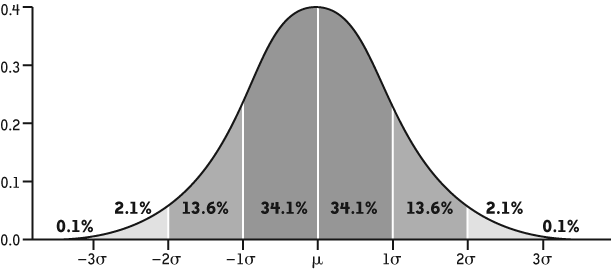
Another common and useful indicator is standard deviation, which refers to the average variance from the calculated mean value. It’s based on the assumption that most data in random, real-life events exhibit a normal distribution, more familiar to most of us from high school as a “bell curve.” The higher the standard deviation, the farther the items of data tend to lie from the mean. Figure 4-1 provides an example courtesy of Wikipedia.

Figure 4-1. Simple bell curve example

In performance testing terms, a high standard deviation can indicate an erratic end-user experience. For example, a transaction may have a calculated mean response time of 40 seconds but a standard deviation of 30 seconds. This would mean that an end user has a high chance of experiencing a response time as low as 25 and as high as 55 seconds for the same activity. You should seek to achieve a small standard deviation.

Nth percentile

Percentiles are used in statistics to determine where a certain percent of results fall. For instance, the 40th percentile is the value at or below which 40 percent of a set of results can be found. Calculating a given percentile for a group of numbers is not straightforward, but your performance testing tool should handle this automatically. All you normally need to do is select the percentile (anywhere from 1 to 100) to eliminate the values you want to ignore.

For example, let’s take the set of numbers from our earlier skewed example (1, 2, 2, 2, 3, 9) and ask for the 90th percentile. This would lie between 3 and 9, so we eliminate the high value 9 from the results. We could then apply our arithmetic mean to the remaining 5 values, giving us the much more representative value of 2 (1 + 2 + 2 + 2 + 3 divided by 5).

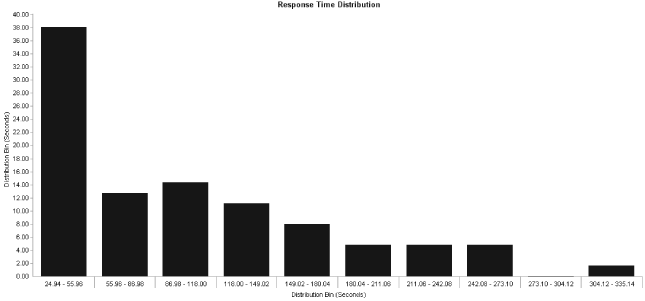
Response-time distribution

Based on the normal distribution model, this is a way of aggregating all the response times collected during a performance test into a series of groups or “buckets.” This distribution is usually rendered as a bar graph, where each bar represents a range of response times and what percentage of transaction iterations fell into that range. You can normally define how many bars you want in the graph and the time range that each bar represents. The Y-axis is simply an indication of measured response time. See Figure 4-2.

Figure 4-2. Response-time distribution

Response-Time Measurement

The first set of data you will normally look at is a measurement of application—or, more correctly, server—response time per transaction. Automated performance test tools typically measure the time it takes for an end user to submit a request to the application and receive a response. If the application fails to respond in the required time, the performance tool will record some form of time-out error. If this situation occurs then it is quite likely that an overload condition has occurred somewhere in the application landscape. We then need to check the server and network KPIs to help us determine where the overload occurred.

Tip

An overload doesn’t always represent a problem with the application. It may simply mean that you need to increase one or more time-out values in the transaction script or the performance test configuration.

Any application time spent exclusively on the client is rendered as periods of think time, which represent the normal delays and hesitations that are part of end-user interaction with a software application. Performance testing tools generally work at the middleware level—that is, under the presentation layer—so they have no concept of events such as clicking on a combo-box and selecting an item unless this action generates traffic on the wire. User activity like this will normally appear in your transaction script as a period of inactivity or “sleep time” and may represent a simple delay to simulate the user digesting what has been displayed on the screen as well as individual or multiple actions of the type just described. If you need to time such activities separately then you may need to combine functional and performance testing tools as part of the same performance test (see Chapter 5).

These think-time delays are not normally included in response time measurement, since your focus is on how long it took for the server to send back a complete response after a request is submitted. Some tools may break this down further by identifying at what point the server started to respond and how long it took to complete sending the response.

Moving on to some examples, the next three figures demonstrate typical response-time data that would be available as part of the output of a performance test. This information is commonly available both in real time (as the test is executing) and as part of the completed test results.

Figure 4-3 depicts simple transaction response time (Y-axis) versus the duration of the performance test (X-axis). On its own this metric tells us little more than the response time behavior for each transaction over the duration of the performance test. If there are any fundamental problems with the application then response-time performance is likely to be bad regardless of the number of virtual users that are active.

Figure 4-3. Transaction response time for the duration of a performance test

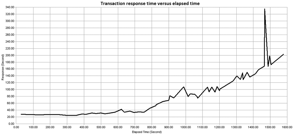
Figure 4-4 shows response time for the same test but this time adding the number of concurrent virtual users at each point. Now you can see the effect of increasing numbers of virtual users on application response time. You would normally expect an increase in response time as more virtual users become active, but this should not vary in lockstep with increasing load.

Figure 4-4. Transaction response time correlated with concurrent users for the duration of a test

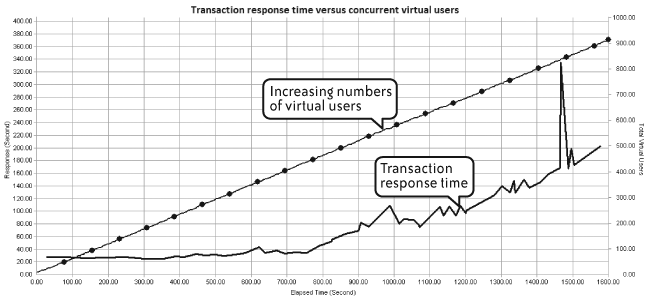
Figure 4-5 builds on the previous two by adding response-time data for the checkpoints that were defined as part of the transaction. As mentioned in Chapter 2, adding checkpoints improves the granularity of the response-time analysis and allows correlation of poor response-time performance with the specific activities of a transaction. The figure shows that the spike in transaction response-time at approximately 1,500 seconds corresponded to an even more dramatic spike in checkpoints but did not correspond to the number of active virtual users.

Figure 4-5. Transaction and checkpoint response time correlated with concurrent users

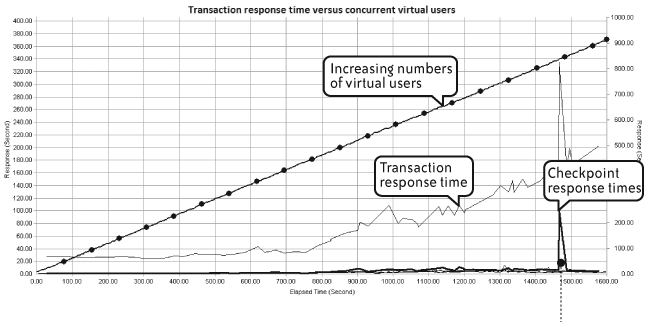
In fact, the response-time spike at about 1,500 seconds was caused by an invalid set of login credentials supplied as part of the transaction input data. This clearly demonstrates the effect that inappropriate data can have on the results of a performance test.

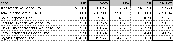
Figure 4-6 provides a tabular view of response time data graphed in Figure 4-5. Here we see references to mean and standard deviation values for the complete transaction and for each checkpoint.

Figure 4-6. Table of response-time data

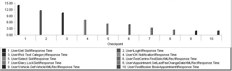
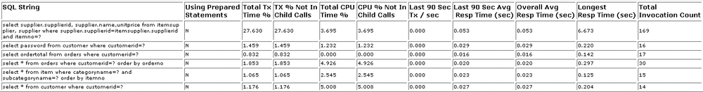
Performance testing tools should provide us with a clear starting point for analysis. For example, Figure 4-7 lists the ten worst-performing checkpoints for all the transactions within a performance test. This sort of graph is useful for highlighting problem areas when there are many checkpoints and transactions.

Figure 4-7. Top ten worst-performing checkpoints

Throughput and Capacity

Next to response time, performance testers are usually most interested in how much data or how many transactions can be handled simultaneously. You can think of this measurement as throughput to emphasize how fast a particular number of transactions are handled or as capacity to emphasize how many transactions can be handled in a particular time period.

Figure 4-8 illustrates transaction throughput per second for the duration of a performance test. This view shows when peak throughput was achieved and whether any significant variation in transaction throughput occurred at any point.

Figure 4-8. Transaction throughput

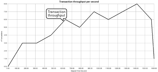
A sudden reduction in transaction throughput invariably indicates problems and may coincide with errors encountered by a virtual user. I have seen this frequently occur when the web server tier reaches its saturation point for incoming requests. Virtual users start to stall while waiting for the web servers to respond, resulting in an attendant drop in transaction throughput. Eventually users will start to time out and fail, however you may find that throughput stabilizes again (albeit at a lower level) once the number of active users is reduced to a level that can be handled by the web servers. If you’re really unlucky, the web or application servers may not be able to recover and all your virtual users will fail.

In short, reduced throughput is a useful indicator of the capacity limitations in the web or application server tier.

Figure 4-9 looks at the number of GET, CONNECT, and POST requests for active concurrent users during a web-based performance test. These values should gradually increase over the duration of the test, as they do in Figure 4-9. Any sudden drop-off, especially when combined with the appearance of virtual user errors, could indicate problems at the web server layer.

Figure 4-9. Concurrent virtual users correlated with web request attempts

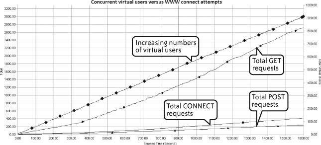
Of course, the web servers are not always the cause of the problem. I have seen many cases where virtual users timed out waiting for a web server response, only to find that the actual problem was a long-running database query that had not yet returned a result to the application or web server tier. This demonstrates the importance of setting up KPI monitoring for all server tiers in the application landscape.

Monitoring Key Performance Indicators (KPIs)

As discussed in Chapter 2, you can determine server and network performance by configuring your monitoring software to observe the behavior of key generic and application-specific performance counters. This monitoring software may be included in or integrated with your automated performance testing tool, or it may be an independent product. Any server and network KPIs configured as part of performance testing requirements fall into this category.

You can use a number of mechanisms to monitor server and network performance, depending on your application technology and the capabilities of your performance testing solution. The following sections divide the tools into categories, describing the most common technologies in each category.

Remote monitoring

These technologies provide server performance data (along with other metrics) to a remote system. That is, the server being tested passes data over the network to the part of your performance testing tool that runs your monitoring software.

The big advantage of using remote monitoring is that you don’t usually need to install any software onto the servers you want to monitor. This circumvents problems with internal security policies that prohibit installation of any software that is not part of the “standard build.” A remote setup also makes it possible to monitor many servers from a single location.

That said, each of these monitoring solutions needs to be activated and correctly configured. You’ll need to be provided with an account that has sufficient privilege to access the monitoring software. You should also be aware that some forms of remote monitoring, particularly SNMP or anything using Remote Procedure Calls (RPC), may be prohibited by site policy because they can compromise security.

Common remote monitoring technologies include the following.

Windows Registry

This provides essentially the same information as Microsoft’s Performance Monitor (Perfmon) application. Most performance testing tools provide this capability. This is the standard source of KPI performance information for Windows operating systems and has been in common use since Windows 2000 was released.

Web-Based Enterprise Management (WBEM)

Web-Based Enterprise Management is a set of systems management technologies developed to unify the management of distributed computing environments. WBEM is based on Internet standards and Distributed Management Task Force (DMTF) open standards: the Common Information Model (CIM) infrastructure and schema, CIM-XML, CIM operations over HTTP, and WS-Management. Although its name suggests that WBEM is web-based, it is not necessarily tied to any particular user interface.

Microsoft has implemented WBEM through their Windows Management Instrumentation (WMI) model. Their lead has been followed by most of the major Unix vendors, such as SUN and HP. This is relevant to performance testing because Windows Registry information is so useful on Windows systems and is universally used as the source for monitoring, WBEM itself is relevant mainly for non-Windows operating systems. Many performance testing tools support Microsoft’s WMI, although you may have to manually create the WMI counters for your particular application and there may be some limitations in each tool’s WMI support.

Simple Network Monitoring Protocol (SNMP)

A misnomer if ever there was one; I don’t think anything is simple about using SNMP. However, this standard has been around in one form or another for many years and can provide just about any kind of information for any network or server device. SNMP relies on the deployment of Management Information Base (MIB) files that contain lists of Object Identifiers (OIDs) to determine what information is available to remote interrogation. For the purposes of performance testing, think of an OID as a counter of the type available from Perfmon. The OID, however, can be a lot more abstract, providing information such as the fan speed in a network switch. There is also a security layer based on the concept of “communities” to control access to information. Therefore, you need to ensure that you can connect to the appropriate community identifier; otherwise you won’t see much. SNMP monitoring is provided by a number of performance tool vendors.

Java Monitoring Interface (JMX)

Java Management Extensions is a Java technology that supplies tools for managing and monitoring applications, system objects, devices (such as printers), and service-oriented networks. Those resources are represented by objects called MBeans (for Managed Beans). JMX is useful mainly when monitoring Java application servers such as IBM WebSphere, ORACLE WebLogic, and JBOSS. JMX support is version-specific, so you need to check which versions are supported by your performance testing solution.

Rstatd

This is a legacy RPC-based utility that has been around in the Unix world for some time. It provides basic kernel-level performance information. This information is commonly provided as a remote monitoring option, although it is subject to the same security scrutiny as SNMP because it uses RPC.

Installed agent

When it isn’t possible to use remote monitoring—perhaps because of network firewall constraints or security policies—your performance testing solution may provide an agent component that can be installed directly onto the servers you wish to monitor. You may still fall foul of internal security and change requests, causing delays or preventing installation of the agent software, but it’s a useful alternative if your performance testing solution offers this capability and the remote monitoring option is not available.

Server KPI Performance

Server KPIs are many and varied. However, two that stand out from the crowd are: how busy the server CPUs are and how much virtual memory is available. These two metrics on their own can tell you a lot about how a particular server is coping with increasing load. Some automated tools provide an expert analysis capability that attempts to identify any anomalies in server performance that relate to an increase in the number of virtual users or transaction response time (e.g., a gradual reduction in available memory in response to an increasing number of virtual users).

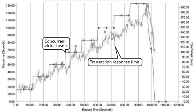
Figure 4-10 demonstrates a common correlation by mapping the number of concurrent virtual users against how busy the server CPU is. These relatively simple views can quickly reveal if a server is under stress. The figure depicts a “ramp-up with step” virtual user injection profile.

Figure 4-10. Concurrent virtual users correlated with database CPU utilization

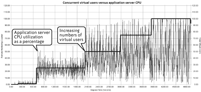
A notable feature of Figure 4-10 is the spike in CPU usage right after each step up in virtual users. For the first couple of steps the CPU soon settles down and handles that number of users better, but as load increases the CPU utilization becomes increasingly intense. Remember that the injection profile you select for your performance test scripts can create periods of artificially high load, especially right after becoming active, so you need to bear this in mind when analyzing test results.

Network KPI Performance

As with server KPIs, any network KPIs instrumented as part of the test configuration should be available afterwards for post-mortem analysis. The following example demonstrates typical network KPI data that would be available as part of the output of a performance test.

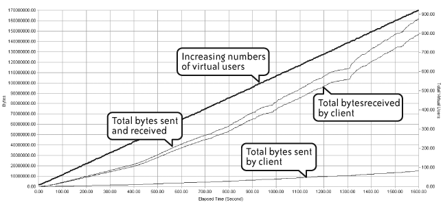
Figure 4-11 correlates concurrent virtual users with various categories of data presented to the network. This sort of view provides insight into the data “footprint” of an application, which can be seen either from the perspective of a single transaction or single user (as may be the case when baselining) or during a multitransaction performance test. This information is useful for estimating the application’s potential impact on network capacity when deployed.

In this example it’s pretty obvious that a lot more data is being received than sent by the client, suggesting that whatever caching mechanism is in place may not be optimally configured.

Figure 4-11. Network byte transfers correlated with concurrent virtual users

Load Injector Performance

Every automated performance test uses one or more workstations or servers as load injectors. It is very important to monitor the stress on these machines as they create increasing numbers of virtual users. As mentioned in Chapter 2, if the load injectors themselves become overloaded then your performance test will no longer represent real-life behavior and so will produce invalid results that lead you astray. Overstressed load injectors don’t necessarily cause the test to fail, but they could easily distort the transaction and data throughput as well as the number of virtual user errors that occur during test execution. Carrying out a dress rehearsal in advance of full-blown testing will help ensure that you have enough injection capacity.

Typical metrics you need to monitor include:

• Percent of CPU utilization

• Amount of free memory

• Page file utilization

• Disk time

• Amount of free disk space

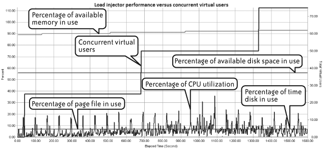
Figure 4-12 offers a typical runtime view of load injector performance monitoring. In this example, disk space utilization is reassuringly stable, and CPU utilization seems to stay within safe bounds even though it fluctuates greatly.

Figure 4-12. Load injector performance monitoring

Root-Cause Analysis

So what are we looking for to determine how our application is performing? Every performance test offers a number of KPIs that can provide the answers.

Tip

Before proceeding with analysis, you might want to adjust the time range of your test data to eliminate the start-up and shutdown periods that can denormalize your statistical information. This also applies if you have been using a “ramp-up with step” injection profile. If each ramp-up step is carried out en masse (e.g., you add 25 users every 15 minutes), then there will be a period of artificial stress immediately after the point of injection that may influence your performance stats (Figure 4-10). After very long test runs, you might also consider thinning the data, reducing the number of data points to make analysis easier. Most automated performance tools offer the option of data thinning.

Scalability and Response Time

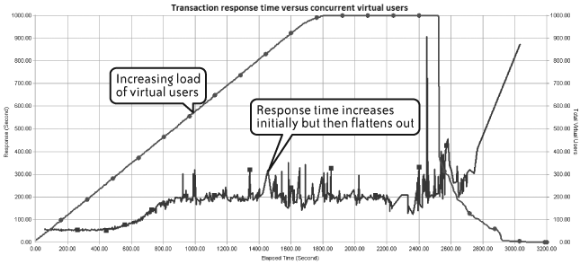
A good model of scalability and response time demonstrates a moderate but acceptable increase in mean response time as virtual user load and transaction throughput increase. A poor model exhibits quite different behavior: as virtual user load increases, response time increases in lockstep and either does not flatten out or starts to become erratic, exhibiting high standard deviations from the mean.

Figure 4-13 shows good scalability. The line representing mean transaction response time increases to a certain point in the test but then gradually flattens out as maximum concurrency is reached. Assuming that the increased response time remains within your performance targets, this is a good result. (The spikes toward the end of the test were caused by termination of the performance test and don’t indicate a sudden application related problem.)

Figure 4-13. Good scalability/response time model

Figures 4-14 and 4-15 demonstrate undesirable response-time behavior. In Figure 4-14, the line representing mean transaction response time closely follows the line representing number of active virtual users until it hits approximately 750. At this point, response time starts to become erratic, indicating a high standard deviation and a potentially bad end-user experience.

Figure 4-14. Poor scalability/response time model

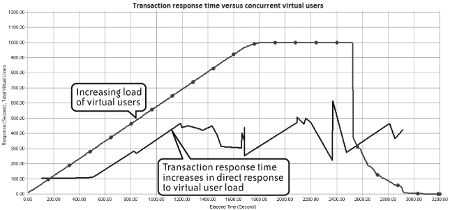
Figure 4-15 demonstrates this same effect in more dramatic fashion. Response time and concurrent virtual users in this example increase almost in lockstep.

Figure 4-15. Consistently worsening scalability/response time model

Digging Deeper

Of course, scalability and response time behavior is only half the story. Once you see a problem, as in Figure 4-14, you need to find the cause. This is where the server and network KPIs come really into play.

Examine the KPI data to see whether any metric correlates with the observed scalability/response time behavior. Some performance testing tools have an autocorrelation feature that provides this information at the end of the test. Other tools require a greater or lesser degree of manual effort to achieve the same result.

The following example demonstrates how it is possible to map server KPI data with scalability and response time information to perform this type of analysis.

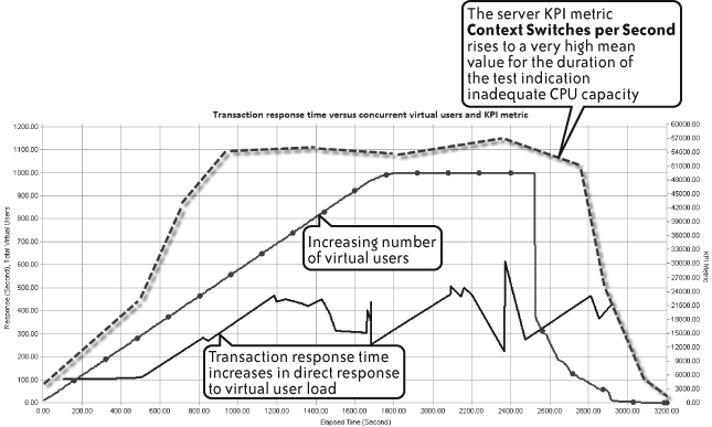
Figure 4-16 builds on Figure 4-14, adding the Windows Server KPI metric called context switches per second. This metric is a good indicator on Windows servers of how well the CPU is handling requests from active threads. This example shows the CPU quickly reaching a high average value, indicating a lack of CPU capacity for the load being applied. This, in turn, is having a negative impact on the ability of the application to scale efficiently and thus on response time.

Figure 4-16. Mapping context switches per second to poor scalability/response time model

Inside the Application Server

In Chapter 2 we discussed setting appropriate server and network KPIs. I suggested defining these as layers, starting from a high-level, generic perspective and then adding others that focus on specific application technologies. One of the more specific KPIs concerned the performance of any application server component present in the application landscape. This type of monitoring lets you look “inside” the application server down to the level of Java or .NET components and methods.

Simple generic monitoring of application servers won’t tell you much if there are problems in the application. In the case of a Java-based application server in a Windows environment, all you’ll see is one or more java.exe processes consuming a lot of memory or CPU. You need to discover which specific component calls are causing the problem

You may also run into the phenomenon of the stalled thread, where an application server component is waiting for a response from another internal component or from another server such as the database host. When this occurs, there is usually no indication of excessive CPU or memory utilization, just slow response time. The cascading nature of these problems makes them difficult to diagnose without detailed application server analysis.

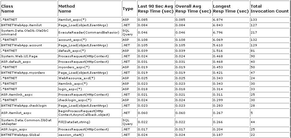
Figures 4-17 and 4-18 present the type of performance data that this analysis provides.

Figure 4-17. Java application server’s worst-performing SQL calls

Figure 4-18. Java application server’s worst-performing methods

Looking for the “Knee”

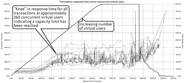
You may find that, at a certain throughput or number of concurrent virtual users during a performance test, the performance testing graph demonstrates a sharp upward trend—known colloquially as a knee—in response time for some or all transactions. This indicates that some capacity limit has been reached within the application landscape and has started to affect application response time.

Figure 4-19 demonstrates this effect during a large-scale multitransaction performance test. At approximately 260 concurrent users, there is a distinct “knee” in the measured response time of all transactions. After you observe this behavior, your next step should be to be look at server and network KPIs at the same point in the performance test. This may, for example, reveal high CPU utilization or insufficient memory on one or more of the application server tiers.

Figure 4-19. “Knee” performance profile indicating that capacity limits have been reached

In this particular example, the application server was found to have high CPU utilization and very high context switching, indicating a lack of CPU capacity for the required load. To fix the problem, the application server was upgraded to a more powerful machine. It is a common strategy to simply throw hardware at a performance problem. This may provide a short-term fix, but it carries a cost and a significant amount of risk that the problem will simply re-appear at a later date. In contrast, a clear understanding of the problem’s cause provides confidence that the resolution path chosen is the correct one.

Dealing with Errors

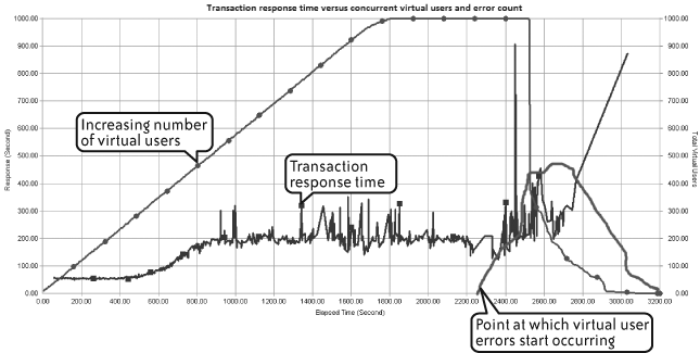
It is most important to examine any errors that occur during a performance test, since these can also indicate hitting some capacity limit within the application landscape. By “errors” I mean virtual user failures, both critical and noncritical. Your job is to find patterns of when these errors start to occur and the rate of further errors occurring after that point. A sudden appearance of a large number of errors may coincide with the knee effect described previously, providing further confirmation that some limit has been reached. Figure 4-20 adds a small line to Figure 4-14 showing the sudden appearance of errors. The errors actually start before the test shows any problem in response time, and they spike about when response time suddenly peaks.

Figure 4-20. Example of errors occurring during a performance test

Baseline Data

The final output from a successful performance testing project should be baseline performance data that can be used when monitoring application performance after deployment. You now have the metrics available that allow you to set realistic performance SLAs for client, network, and server (CNS) monitoring of the application in the live environment. These metrics can form a key input to your Information Technology Service Management (ITSM) implementation, particularly with regard to End User Experience (EUE) monitoring (see The IT Business Value Curve” in Chapter 1).

Analysis Checklist

To help you adopt a consistent approach to analyzing the results of a performance test both in real time and after execution, here is another checklist. There’s some overlap with the checklist from Chapter 3, but the focus here is on analysis rather than execution. For convenience, I have repeated this information as part of the quick-reference guides in Appendix B.

Pre-Test Tasks

• Make sure that you have configured the appropriate server, application server, and network KPIs. If you are planning to use installed agents instead of remote monitoring, make sure there will be no obstacles to installing and configuring the agent software on the servers.

• Make sure that you have decided on the final mix of performance tests to execute. As discussed in Chapter 3, this commonly includes baseline tests, load tests, and isolation tests of any errors found, followed by soak and stress tests.

• Make sure that you can access the application from your injectors! You’d be surprised how often a performance test has failed to start because of poor application connectivity. This can also be a problem during test execution: testers may be surprised to see a test that was running smoothly suddenly fail completely, only to find after much scratching of heads that the network team has decided to do some unscheduled “housekeeping.”

• If your performance testing tool provides the capability, set any automatic thresholds for performance targets as part of your performance test configuration. This capability may simply count the number of times a threshold is breached during the test, and it may also be able to control the behavior of the performance test as a function of the number of threshold breaches that occur—for example, more than ten breaches of a given threshold could terminate the test.

• If your performance testing tool provides the capability, configure autocorrelation between transaction response time, concurrent virtual users, and server or network KPI metrics. This extremely useful feature is often included in recent generations of performance testing software. Essentially, it will automatically look for (undesirable) changes in KPIs or transaction response time in relation to increasing virtual user load or transaction throughput. It’s up to you to decide what constitutes “undesirable” by setting thresholds for the KPIs you are monitoring, although the tool should provide some guidance.

• If you are using third-party tools to provide some or all of your KPI monitoring, make sure that they are correctly configured before running any tests. Ideally, include them in your dress rehearsal and examine their output to make sure it’s what you expect. I have been caught running long duration tests only to find that the KPI data collection was wrongly configured or even corrupted!

• You frequently need to integrate third-party data with the output of your performance testing tool. Some tools allow you to automatically import and correlate data from external sources. If you’re not fortunate enough to have this option, then you’ll need to come up with a mechanism to do it efficiently yourself. I tend to use MS Excel or even MS Visio, as both are good at manipulating data. But be aware that this can be a very time-consuming task.

Tasks During Test Execution

• At this stage, your tool is doing the work. You need only periodically examine the performance of your load injectors to ensure that they are not becoming stressed. The dress rehearsal carried out before starting the test should have provided you with confidence that enough injection capacity is available, but it’s best not to make assumptions.

• Make sure you document every test that you execute. At a minimum, record the following information:

  • The name of the performance test execution file and the date and time of execution.

  • A brief description of what the test comprised. (This also goes into the test itself, if the performance testing tool I’m using allows it.)

  • If relevant, the name of the results file associated with the current test execution.

  • Any input data files associated with the performance test and which transactions they relate to.

  • A brief description of any problems that occurred during the test.

  It’s easy to lose track of how many tests you’ve executed and what each test represented. If your performance testing tool allows you to annotate the test configuration with comments, make use of this facility to include whatever information will help you to easily identify the test run. Also make sure that you document which test result files relate to each execution of a particular performance test. Some performance testing tools store the results separately from other test assets, and the last thing you want when preparing your report is to wade through dozens of sets of data looking for the one you need. (I speak from experience on this one!)

  Finally, if your performance testing tool allows you to store test assets on a project basis, this can greatly simplify the process of organizing and accessing test results.

• Things to look out for during execution include the following:

  The sudden appearance of errors

  This frequently indicates that some limit has been reached within the application landscape. If your test is data-driven, it can also mean you’ve run out of data. It’s worth determining whether the errors relate to a certain number of active virtual users. Some performance tools allow manual intervention to selectively reduce the number of active users for a troublesome transaction. You may find that errors appear when, say, 51 users are active, but by dropping back to 50 users the errors go away.

  Note

  Sudden errors can also indicate a problem with the operating system’s default settings. I recall a project where the application mid-tier was deployed on a number of blade servers running Sun Solaris Unix. The performance tests persistently failed at a certain number of active users, although there was nothing to indicate a lack of capacity from the server KPI monitoring we configured. A search through system log files revealed that the problem was an operating system limit on the number of open file handles for a single user session. When we increased the limit from 250 to 500, the problem went away.

  A sudden drop in transaction throughput

  This is a classic sign of trouble, particularly with web applications where the virtual users wait for a response from the web server. If the problem is critical enough, the queue of waiting users will eventually exceed the time-out threshold for server responses and the test will exit. Don’t immediately assume that the web server layer is the problem; it could just as easily be the application server or database tier. You may also find that the problem resolves itself when a certain number of users have dropped out of the test, identifying another capacity limitation in the application landscape. If your application is using links to external systems, check to ensure that none of these links is the cause of the problem.

  An ongoing reduction in available server memory

  You would expect available memory to decrease as more and more virtual users become active, but if the decrease continues after all users are active then you may have a memory leak. Application problems that hog memory should reveal themselves pretty quickly, but only a soak test can reveal more subtle problems with releasing memory. This is a particular problem with application servers, and it confirms the value of providing analysis down to the component and method level.

  Panic phone calls from infrastructure staff

  Seriously! I’ve been at testing engagements where the live system was accidentally caught up in the performance testing process. This is most common with web applications, where it’s all too easy to target the wrong URL.

Post-Test Tasks

• Once a performance test has completed—whatever the outcome—make sure that you collect all relevant data for each test execution. It is easy to overlook important data, only to find it missing when you begin your analysis. Most performance tools collect this information automatically at the end of each test execution, but if you’re relying on other third-party tools to provide monitoring data then make sure you preserve the files you need.

• It’s good practice to back up all testing resources (e.g., scripts, input data files, test results) onto a separate archive, because you never know when you may need to refer back to a particular test run.

• When producing your report, make sure that you map results to the performance targets that were set as part of the pre-test requirements capture phase. Meaningful analysis is possible only if you have a common frame of reference.

Summary

This chapter has served to demonstrate the sort of information provided by automated performance testing tools and how to go about effective root-cause analysis. The next chapter looks at how different application technologies affect your approach to performance testing.