View Updating and Relational Theory

Chapter 1. A Motivating Example

Example is always more efficacious than precept

— Samuel Johnson:

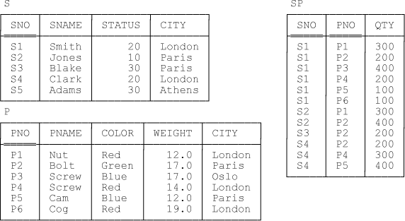
Examples throughout this book are based for the most part on the familiar (not to say hackneyed) suppliers-and-parts database. I apologize for dragging out this old warhorse yet one more time, but as I’ve said elsewhere, I believe using the same example in a variety of different publications can be a help, not a hindrance, in learning. In SQL terms,^[4] the database contains three tables—more specifically, three base tables—called S (“suppliers”), P (“parts”), and SP (“shipments”), respectively. Sample values are shown in Figure 1-1.

Figure 1-1. The suppliers-and-parts database—sample values

The semantics (in outline) are as follows:

• Table S represents suppliers under contract. Each supplier has one supplier number (SNO), unique to that supplier; one name (SNAME), not necessarily unique (though the sample values shown in Figure 1-1 do happen to be unique); one status value (STATUS); and one location (CITY). Note: In the rest of this book I’ll abbreviate “suppliers under contract,” most of the time, to just suppliers.

• Table P represents kinds of parts. Each kind of part has one part number (PNO), which is unique; one name (PNAME); one color (COLOR); one weight (WEIGHT); and one location where parts of that kind are stored (CITY). Note: In the rest of this book I’ll abbreviate “kinds of parts,” most of the time, to just parts.

• Table SP represents shipments—it shows which parts are shipped, or supplied, by which suppliers. Each shipment has one supplier number (SNO); one part number (PNO); and one quantity (QTY). Also, there’s at most one shipment at any given time for a given supplier and given part, and so the combination of supplier number and part number is unique to any given shipment. Note: In the rest of this book I’ll assume QTY values are always greater than zero.

Now I want to focus on table S specifically; for the rest of this chapter, in fact, I’ll mostly ignore tables P and SP, except for an occasional remark here and there. Here’s an SQL definition for that table S:

CREATE TABLE S
  ( SNO    VARCHAR(5)  NOT NULL ,
    SNAME  VARCHAR(25) NOT NULL ,
    STATUS INTEGER     NOT NULL ,
    CITY   VARCHAR(20) NOT NULL ,
    UNIQUE ( SNO ) ) ;

As I’ve said, table S is a base table, but of course we can define any number of views “on top of” that base table. Here are a couple of examples—LS (“London suppliers”) and NLS (“non London suppliers”):

CREATE VIEW LS /* London suppliers */ AS
  ( SELECT SNO , SNAME , STATUS , CITY
    FROM   S
    WHERE  CITY = 'London' ) ;

CREATE VIEW NLS /* non London suppliers */ AS
  ( SELECT SNO , SNAME , STATUS , CITY
    FROM   S
    WHERE  CITY <> 'London' ) ;

Sample values for these views corresponding to the value of table S in Figure 1-1 are shown in Figure 1-2.

Figure 1-2. Views LS and NLS—sample values

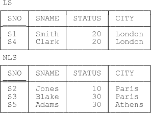
Views LS and NLS are the ones I want to use in this initial chapter as the basis for my motivating example. In essence, what I want to do with that example is try to give you some preliminary idea as to why I believe that—contrary to popular opinion and most conventional wisdom in this area—all views are updatable. (Note, however, that I must immediately qualify this very strong claim by making it clear that I’m necessarily speaking rather loosely at this stage. Later chapters will elaborate.)

The Principle of Interchangeability

So far, then, table S is a base table and tables LS and NLS are views. Observe now, however, that it could have been the other way around—that is, I could have made LS and NLS base tables and S a view, like this:

CREATE TABLE LS
  ( SNO    VARCHAR(5)  NOT NULL ,
    SNAME  VARCHAR(25) NOT NULL ,
    STATUS INTEGER     NOT NULL ,
    CITY   VARCHAR(20) NOT NULL ,
    UNIQUE ( SNO ) ) ;

CREATE TABLE NLS
  ( SNO    VARCHAR(5)  NOT NULL ,
    SNAME  VARCHAR(25) NOT NULL ,
    STATUS INTEGER     NOT NULL ,
    CITY   VARCHAR(20) NOT NULL ,
    UNIQUE ( SNO ) ) ;

CREATE VIEW S AS
  ( SELECT SNO , SNAME , STATUS , CITY
    FROM   LS
    UNION
    SELECT SNO , SNAME , STATUS , CITY
    FROM   NLS ) ;

Note: In order to guarantee that this design is formally equivalent to the original one, I should really state, and have the DBMS enforce, certain integrity constraints—including in particular constraints to the effect that every CITY value in LS is London and no CITY value in NLS is—but I want to ignore such details for the moment. I’ll have a lot more to say about such matters in a little while, I promise you.

Anyway, the message of the example is that, in general, which tables are base ones and which ones are views is arbitrary (at least from a formal point of view). In other words, in the case at hand, we could design the database in at least two different ways—ways, that is, that are logically distinct but information equivalent. (By information equivalent here, I mean the two designs represent the same information, implying among other things that for any query on one, there’s a logically equivalent query on the other. Chapter 3 elaborates on this concept.) And The Principle of Interchangeability is a logical consequence of such considerations:

• Definition: The Principle of Interchangeability states that there must be no arbitrary and unnecessary distinctions between base tables and views; in other words, views should—as far as possible—“look and feel” just like base tables so far as users are concerned.

  Here are some implications of this principle:

• As I’ve already suggested, views are subject to integrity constraints, just like base tables. (We usually think of integrity constraints as applying to base tables specifically, but The Principle of Interchangeability shows this position isn’t really tenable.)

• In particular, views have keys (and so I ought really to have included some key specifications in my view definitions; unfortunately, however, SQL doesn’t permit such specifications).^[5] They might also have foreign keys, and foreign keys might refer to them.

• Many SQL products, and the SQL standard, provide some kind of “row ID” feature (in the standard, that feature goes by the name of REF types and reference values). If that feature is available for base tables but not for views—which in practice is quite likely—then it clearly violates The Principle of Interchangeability.

• Perhaps most important of all, we must be able to update views—because if not, then that fact in itself would constitute the clearest possible violation of The Principle of Interchangeability.

Base Tables Only: Constraints

One thing that follows from The Principle of Interchangeability is that the behavior of tables S, LS, and NLS shouldn’t depend on which if any are base tables and which if any are views. Until further notice, therefore, let’s suppose they’re all base tables:

CREATE TABLE S   ( ... , UNIQUE ( SNO ) ) ;
CREATE TABLE LS  ( ... , UNIQUE ( SNO ) ) ;
CREATE TABLE NLS ( ... , UNIQUE ( SNO ) ) ;

Now, these tables, like all tables, are clearly subject to a number of constraints. Unfortunately, most of those constraints are quite awkward to formulate in SQL, so I’ll content myself for present purposes with stating them in natural language only (and pretty informal natural language at that, for the most part). Here they are:

• {SNO} is a key for each of the tables; also, {SNO} in each of tables LS and NLS is a foreign key, referencing the key {SNO} in table S. Note: For an explanation of why I use braces “{” and “}” here, please refer to SQL and Relational Theory.^[6]

• At any given time, table LS is equal to that restriction of table S where the CITY value is London, and table NLS is equal to that restriction of table S where the CITY value isn’t London. Moreover, every row of table LS has CITY value London,^[7] and no row of table NLS does.

• At any given time, table S is equal to the union of tables LS and NLS; moreover, that union is disjoint (i.e., the corresponding intersection is empty)—no row in S appears in both LS and NLS. To spell the point out in detail: Every row in S also appears in exactly one of LS and NLS, and every row in either LS or NLS also appears in S.

• Finally, the previous constraint and the constraint that {SNO} is a key for all three tables, taken together, imply that every supplier number (not just every row) in S also appears in exactly one of LS and NLS, and every supplier number in either LS or NLS also appears in S.

Of course, as the immediately preceding bullet point illustrates, the foregoing constraints aren’t all independent of one another—some of them are logical consequences of others.

Base Tables Only: Compensatory Actions

Now, in order to ensure that the constraints outlined in the previous section continue to hold when certain updates are done, certain compensatory actions need to be in effect. In general, a compensatory action—also known as a compensating action—is an additional update (over and above some update explicitly requested by the user) that’s performed automatically by the DBMS, precisely in order to avoid some integrity violation that might otherwise occur.^[8] Cascade delete is a typical example.^[9] In the case at hand, in fact, it should be clear that cascading is exactly what we need to deal with DELETE operations in particular. To be specific, deleting rows from either LS or NLS clearly needs to cascade to cause those same rows to be deleted from S. So we might imagine a couple of compensatory actions—actually cascade delete rules—that look something like this (hypothetical syntax):

ON DELETE d FROM LS : DELETE d FROM S ;

ON DELETE d FROM NLS : DELETE d FROM S ;

Likewise, deleting rows from S clearly needs to cascade to cause those same rows to be deleted from whichever of LS or NLS they appear in:

ON DELETE d FROM S : DELETE ( d WHERE CITY = 'London' ) FROM LS ,
                     DELETE ( d WHERE CITY <> 'London' ) FROM NLS ;

As an aside, I remark that, given that an attempt to delete a nonexistent row has no effect—or so I’m going to assume, at any rate—we could replace each of the expressions in parentheses in the foregoing rule by just d. However, the expressions in parentheses are perhaps preferable, at least inasmuch as they’re clearly more specific.

Analogously, we’ll need some compensatory actions (“cascade insert rules”) for INSERT operations:

ON INSERT i INTO LS : INSERT i INTO S ;

ON INSERT i INTO NLS : INSERT i INTO S ;

ON INSERT i INTO S : INSERT ( i WHERE CITY = 'London' ) INTO LS ,
                     INSERT ( i WHERE CITY <> 'London' ) INTO NLS ;

Note: The concept of cascade insert doesn’t usually arise in connection with foreign key constraints, of course, but that’s no reason not to support such a concept in general. More important, don’t get the idea that compensatory actions must always take the form of simple cascades. While the ones discussed in this introductory chapter do all happen to take that form, more complicated cases are likely to require actions of some less straightforward form, as we’ll see in later chapters.

As for UPDATE operations, they can be regarded, at least in the case at hand, as a DELETE and an INSERT taken in combination; as a consequence, the necessary compensatory actions are just a combination of the corresponding delete and insert actions, loosely speaking. For example, consider the following UPDATE on table S:

UPDATE S
SET    CITY = 'Oslo'
WHERE  SNO = 'S1' ;

What happens here is this:

1. The existing row for supplier S1 is deleted from table S and a new row for that supplier, with CITY value Oslo, is inserted into that same table.

2. The existing row for supplier S1 is deleted from table LS as well, thanks to the cascade delete rule from S to LS, and the new row for that supplier, with CITY value Oslo, is inserted into table NLS as well, thanks to the cascade insert rule from S to NLS. In other words, the row for supplier S1 has “migrated” from table LS to table NLS! (Of course, here I’m speaking very loosely indeed.)

   Suppose now that the original UPDATE had been directed at table LS rather than table S:

UPDATE LS
SET    CITY = 'Oslo'
WHERE  SNO = 'S1' ;

Now what happens is this:

1. The existing row for supplier S1 is deleted from table LS.

2. An attempt is made to insert a new row for supplier S1, with CITY value Oslo, into table LS. That attempt fails, however, because it violates the constraint on table LS that the CITY value in that table must always be London. So the update fails overall; the previous step (viz., deleting the original row for supplier S1 from LS) is undone, and the net effect is that the database remains unchanged.

Views: Constraints and Compensatory Actions

Now I come to the real point of this chapter: Everything I’ve said in the previous two sections applies pretty much unchanged if some or all of the tables concerned are views. For example, suppose as we originally did that S is a base table and LS and NLS are views:

CREATE TABLE S      ( .............. , UNIQUE ( SNO ) ) ;
CREATE VIEW  LS  AS ( SELECT ... WHERE CITY = 'London' ) ;
CREATE VIEW  NLS AS ( SELECT ... WHERE CITY <> 'London' ) ;

Now consider a user who sees only views LS and NLS, but wants to be able to behave as if those views were actually base tables. As far as that user is concerned, then, those tables have semantics as follows:

LS: Supplier SNO is under contract, is named SNAME, has status STATUS, and is located in city CITY (which is London).

NLS: Supplier SNO is under contract, is named SNAME, has status STATUS, and is located in city CITY (which is not London).

That same user will also be aware of the following constraints (note that these constraints make no mention of table S, because the user in question doesn’t even know table S exists):

• {SNO} is a key for both LS and NLS.

• Every row in LS has CITY value London, and no row in NLS does.

• No supplier number appears in both LS and NLS.

However, that user won’t be aware of any compensatory actions as such, precisely because he or she isn’t aware that LS and NLS are actually views of S; indeed, as I’ve already said, the user isn’t even aware of the existence of S (which is why that user is also unaware of the constraint to the effect that the union of LS and NLS is equal to S). But updates by that user on LS and NLS will all work as far as that user is concerned exactly as if LS and NLS really were base tables. Also, of course, updates by that user on LS and NLS will have the appropriate effects on S, even though those effects won’t be directly visible to that user.

There’s No Magic

Now consider a user who sees only, say, view LS (i.e., not view NLS and not base table S). Presumably this user still wants to be able to behave as if LS were a base table. Of course, this user will certainly know the semantics of that table—

LS: Supplier SNO is under contract, is named SNAME, has status STATUS, and is located in city CITY (which is London).

—and will also be aware of the following constraints:

• {SNO} is a key for LS.

• Every row in LS has CITY value London.

Clearly, this user can’t be allowed to insert rows into this table—nor to update supplier numbers within this table—because such operations have the potential to violate constraints of which this user is unaware (and must be unaware).^[10] But if LS really were a base table, it would surely be possible to insert rows into it, wouldn’t it? Indeed, if it weren’t, then the table would always be empty! So doesn’t the foregoing state of affairs constitute a violation of The Principle of Interchangeability?

In fact it does not. While it’s true that this particular user can’t be allowed to insert rows into the table, that’s not the same as saying no user is allowed to do so. The basic reason why this particular user can’t insert rows into LS is that this user is seeing only part of the picture, as it were. Contrast a user who does see both LS and NLS, which in combination are information equivalent to the original table S; as we saw in the previous section, such a user certainly can insert rows into LS (and/or NLS). But the user who sees only LS is seeing something that isn’t information equivalent to the original table S, and so it’s only to be expected that there’ll be certain operations that he or she can’t be allowed to do.

In closing, it’s worth pointing out that even here there are parallels with the situation in which all tables involved really are base tables. That is, even when the tables in question are all base tables, it’ll sometimes be the case that certain users will be prohibited from performing certain updates on certain tables. By way of example, consider a user who sees only base table SP and not base table S. Like the user who sees only table LS, that user can’t be allowed to perform insert operations, because such operations have the potential to violate constraints of which that user is unaware (and must be unaware)—to be specific, the foreign key constraints from SP to tables S and P.

Concluding Remarks

This brings me to the end of the discussion of the motivating example. Now, that example is extremely simple, and the conclusions I’ve drawn from it are perhaps all very obvious; but what I’m suggesting is that thinking of views as base tables “living alongside” the tables in terms of which they’re defined is a fruitful way to think about the view updating problem in general—indeed, not just a fruitful way, but a way I believe is logically correct.^[11] The overall idea is thus as follows:

1. The view defining expressions imply certain constraints. For example, the view defining expression for view LS (“London suppliers”) implies a constraint to the effect that LS is equal to that restriction of table S where the CITY value is London.

2. Such constraints in turn imply certain compensatory actions (i.e., actions that need to be performed, over and above updates that are explicitly requested by the user, in order to avoid some integrity violation that might otherwise occur). For example, the constraints on tables S, LS, and NLS imply certain cascade deletes and cascade inserts, as we’ve seen.

By the way, I’d really like to stress this latter point—the point, that is, that it should be possible for the compensatory actions that apply in a given situation to be determined by the DBMS from the pertinent view defining expression. In other words, what I’m not suggesting is that such actions need to be specified explicitly, thereby imposing yet another administrative burden on the already overworked DBA.^[12] But this issue, like many others I’ve touched on briefly in this introductory chapter, will be explored in more detail in later parts of the book.

In closing, let me suggest that if (like most people) you skipped the preface and started straight in on this first chapter, now would be a good time to go back and read the preface, before you move on to the next chapter. Among other things, the preface includes an outline of the structure of the book overall. It also spells out certain important technical assumptions that I’ll be relying on in the chapters to come, and hence that you need to be aware of.

---

^[4] I use SQL and SQL-style syntax in this introductory chapter for reasons of familiarity, despite the fact that it’s not really to my taste, and (more to the point, perhaps) despite the fact that it actually makes the motivating example harder to explain properly.

^[5] Throughout this book I use the term key, unqualified, to mean a candidate key, not necessarily a primary key specifically. In fact, Tutorial D—see Chapter 2—has no syntax for distinguishing between primary and other keys. For reasons of familiarity, however, I use double underlining in figures like Figure 1-1 to suggest that the attributes so underlined can be thought of as primary key attributes, if you like.

^[6] I remind you from the preface that throughout this book I use “SQL and Relational Theory” as an abbreviated form of reference to my book SQL and Relational Theory: How to Write Accurate SQL Code (2nd edition, O’Reilly, 2012).

^[7] Precisely because of this fact, a more realistic version of view LS would probably drop the CITY attribute. I choose not to do so here, in order to keep the example simple.

^[8] One reviewer asked why I chose the term compensatory action for this construct. Well, I should have thought the answer was obvious, but in case it isn’t, let me spell it out: The reason I call such actions “compensatory” is because they cause a second update to be done to compensate for the effects of the first (speaking a trifle loosely, of course).

^[9] Cascade delete is usually thought of as applying to foreign key constraints specifically; however, the concept of compensatory actions is actually more general and applies to constraints of many kinds.

^[10] I suppose the user might be allowed to perform such operations if he or she is also prepared to accept occasional error messages to the effect that an operation is rejected simply “because the system says so,” without further explanation. See Chapter 4 for further discussion of this point.

^[11] Acknowledgments here to David McGoveran, who first got me thinking along these lines several years ago.

^[12] DBA = database administrator.