VLSI Digital Signal Processing Systems: Design and Implementation

11.3    STATE VARIABLE DESCRIPTION OF DIGITAL FILTERS

Consider the signal flow graph (SFG) of an N-th order digital filter in Fig. 11.5. We can represent this filter in the following recursive matrix form,

The boldfaced letters imply a vector or a matrix. In the above representation x is the state vector, u is the input, and y is the output of the filter; x, b, and c are N × 1 column vectors; A is N × N matrix; d, u and y are scalars. Let f_i(n) be the unit-sample response from the input u(n) to the state x_i(n) and let g_i(n) be the unit-sample response from the state x_i(n) to the output y_i(n). To avoid internal overflow, it is necessary to scale the inputs to multipliers. Since the signals x(n) are inputs to multipliers in Fig. 11.5, we need to compute f(n) for scaling. Conversely, to find the noise variance at the output, it is necessary to find the unit-sample response from the location of the noise source e(n) to y(n). Thus g(n) represents the unit-sample response of the noise transfer function except for a delay, which has no effect on the output noise variance.

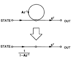
Fig. 11.6    Signal flow graph of g(n).

From the SFG of Fig. 11.5 we can write,

Then we can write the z-transform of ...