An applied introduction to generative adversarial networks

Most of the artificial intelligence (AI) successes in recent years have occurred in narrowly defined problems such as image classification, computer vision, speech recognition, and machine translation, powered by the availability of large data sets, incredibly powerful computers, and supervised learning algorithms.

However, general artificial intelligence—the holy grail of AI research—remains a far-off goal, one that will take decades to achieve. Many in the AI community believe major advances in unsupervised learning—the ability to learn from data without any labels—holds the key to general artificial intelligence.

What are generative adversarial networks?

One major advance in unsupervised learning has been the advent of generative adversarial networks (GANs), introduced by Ian Goodfellow and his fellow researchers at the University of Montreal in 2014. GANs have many applications; for example, we can use GANs to create near-realistic synthetic data, such as images and speech, or perform anomaly detection.

In GANs, we have two neural networks. One network—known as the “generator”—generates data based on a model data distribution it has created using samples of real data it has received. The other network—known as the “discriminator”—discriminates between the data created by the generator and data from the true data distribution.

As a simple analogy, the generator is the counterfeiter, and the discriminator is the police trying to identify the forgery. The two networks are locked in a zero-sum game. The generator is trying to fool the discriminator into thinking the synthetic data comes from the true data distribution, and the discriminator is trying to call out the synthetic data as fake.

GANs are unsupervised learning algorithms because the generator can learn the underlying structure of the true data distribution even when there are no labels. It learns the underlying structure by using a number of parameters significantly smaller than the amount of data it has trained on. This constraint forces the generator to efficiently capture the most salient aspects of the true data distribution.

This is similar to the representation learning that occurs in deep learning. Each hidden layer in the neutral network of a generator captures a representation of the underlying data—starting very simply—and subsequent layers pick up more complicated representations by building on the simpler preceding layers. Using all these layers together, the generator learns the underlying structure of the data and, using what it has learned, the generator attempts to create synthetic data that is nearly identical to the true data distribution. If the generator has captured the essence of the true data distribution, the synthetic data will appear real.

Real-world applications of GANs

For real-world applications, both the generator and the discriminator are valuable. If the objective is to generate a lot of new training examples to help supplement existing training data—for example, to improve accuracy on an image recognition task—we can use the generator to create a lot of synthetic data, add the new synthetic data to the original training data, and then run a supervised machine learning model on the now much larger data set.

If the objective is to identify anomalies—for example, to detect fraud, hacking, or other suspicious behavior—we can use the discriminator to score each instance in the real data. The instances that the discriminator ranks as “likely synthetic” will be the most anomalous instances and also the ones most likely to represent malicious behavior.

A simple one-dimensional data distribution

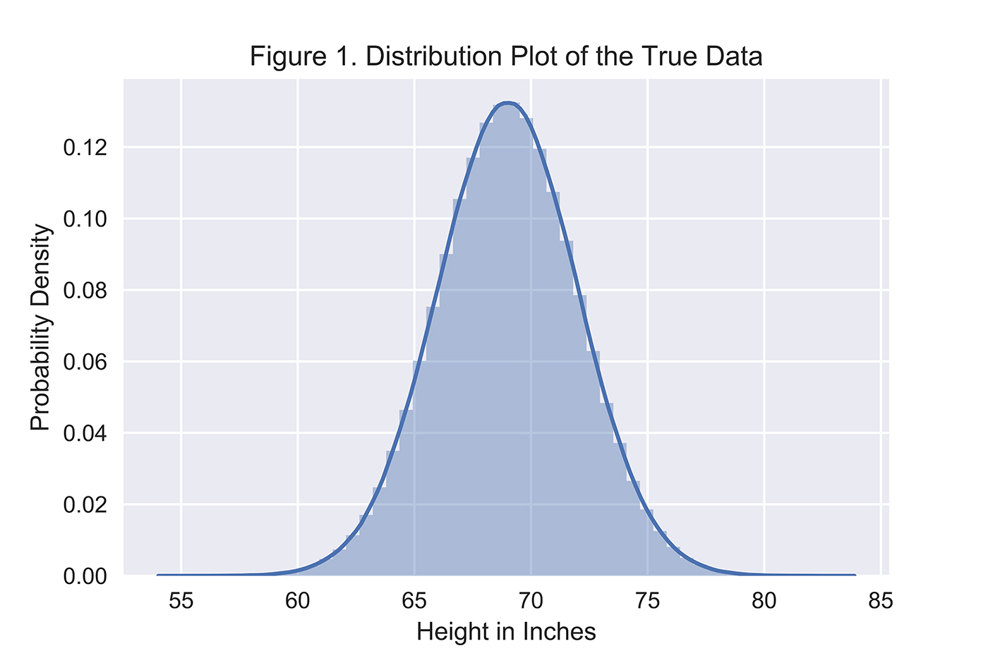
Let’s consider a simple example: assume we have a true data distribution of heights for males in the United States, which is normally distributed (Figure 1) with a mean of 69 inches and a standard deviation of 3 inches.

The generator does not know the true underlying distribution of heights but will try to model this distribution based on actual height data that it receives. The more data it receives, the better its model distribution will be. The generator will then use this model distribution to generate synthetic heights, and the discriminator will try to identify which of the heights are actual versus synthetic.

Set up the neural networks

For the generator, we will use a neural network with five hidden layers, each with 10 hidden nodes. At each hidden layer, we will perform a linear transformation and pass it through a nonlinearity (hyperbolic tangent function). To speed up the training, we will perform batch normalization, and, to address overfitting, we will use dropout. After the final hidden layer, we will perform a final linear transformation, leaving us with a one-dimensional output.

For the discriminator, we will use a neural network with three hidden layers, each with two hidden nodes. As with the generator, at each hidden layer we will perform a linear transformation and pass it through a nonlinearity (hyperbolic tangent function). Given the simplicity of this neural network, we will not perform batch normalization or use dropout. After the final hidden layer, we will perform a final linear transformation and pass it through the sigmoid function, leaving us with a one-dimensional output that can be interpreted as the confidence the discriminator has in calling out a forgery.

Using its neural network, the generator G will attempt to map actual heights—z₁, z₂, z₃, …, z_m, where m is the total number of samples—to x₁, x₂, x₃, x₄, …, x_m such that x_i = G(z_i). z_i comes from the true height data distribution. x_i is the newly generated synthetic data.

If the generator performs well, the model distribution it generates will be nearly identical to the true underlying distribution of heights. In other words, x_i will be dense where z_i is dense, and x_i will be sparse where z_i is sparse.

Define the objective functions

The discriminator D will take in input data x and determine whether x belongs to the true data distribution. If x is from the true data distribution, we want D(x) to be maximized. If x is synthetic—from now on referred to as x’—we want D(x’) to be minimized.

The objective function for D is: log(D(x)) + log(1 – D(x’)), where x is from the true data distribution (i.e., z_i) and x’ is synthetic data x_i generated from G(z_i). The discriminator will try to maximize this function.

The objective function for G is: log(D(x’)), where x’ is synthetic data x_i generated from G(z_i). The better the generator is at fooling the discriminator, the higher the value of this function will be.

Define the optimizer and set the hyperparameters

We will use a simple gradient descent optimizer for this problem with an initial learning rate of 0.005. This learning rate will decay every 100 steps we take. We will use a batch size of 200 and train for 10,000 epochs.

Start training and evaluate the results

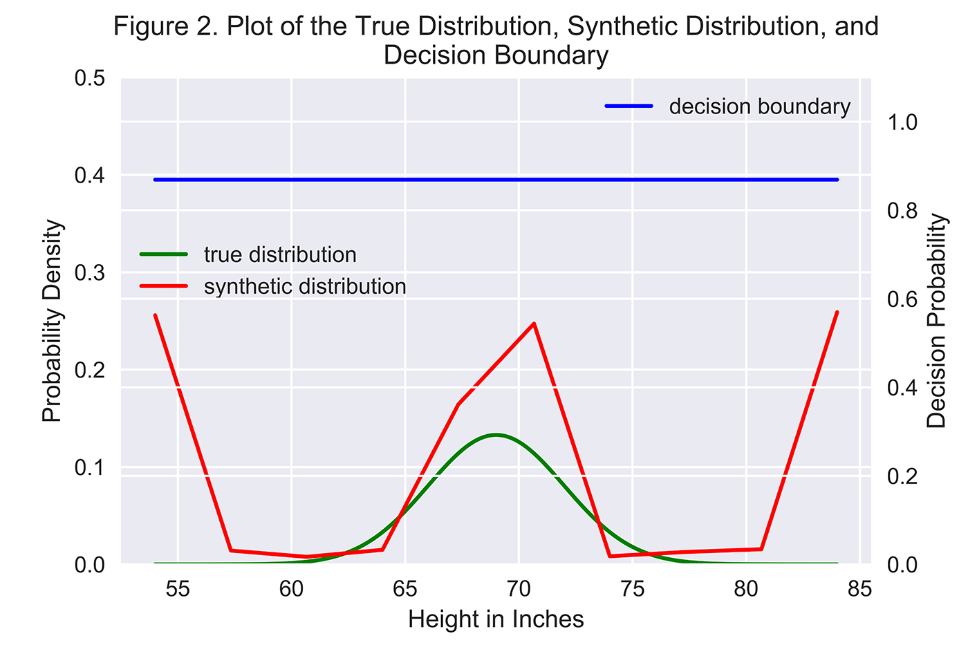
To evaluate the results, let’s plot the true data distribution and the synthetic data distribution along with the decision boundary of the discriminator. If the decision boundary is at or near 0.50, the discriminator cannot tell the difference between the real data and the synthetic data—it is just randomly guessing at this point. If the decision boundary is much higher or lower than 0.50, the discriminator is much more confident at catching the forgery.

In Figure 2, the decision boundary (measured on the right-hand scale) is above 0.80, which means the discriminator is very good at identifying the synthetic data. But, the generator gets better over time—it does a good job of capturing where the center of the distribution lies but still struggles with modeling the tail ends of the true distribution.

In this simple example, the generator is good, but the discriminator is much better. To improve the generator, we can introduce more advanced techniques, including feature matching and minibatch discrimination, both of which we will explore in a future article.

The power and potential of GANs

Instead of modeling simple one-dimensional data sets, we can use GANs to create synthetic images and speech to supplement existing real data sets (e.g., to train machine learning models), or, perhaps for more nefarious purposes, to create counterfeit documents and art and impersonate other people.

We can also use GANs to perform anomaly detection by using the discriminator to detect probabilistically rare data (outliers) from more normal data.

We are still in the very early stages of GANs, so a lot of work remains. But, with GANs, artificial intelligence agents may be able to generate synthetic data that is virtually indistinguishable from real data. This will bring AI one step closer to passing the Turing Test, in which it exhibits behavior that is nearly identical to that of a human—a la Ex Machina and Westworld.

In other words, GANs may hold the key to solving one of the greatest feats in the field of artificial intelligence.