
 Whirl (source: Pixabay)
 In our previous notebooks, we used a deep learning technique called convolution neural network (CNN) to classify text and images. Even though CNN is a powerful technique, it cannot learn temporal features from an input sequence such as audio and text. Moreover, CNN is designed to learn spatial features with a fixed-length convolution kernel. These types of neural networks are called feedforward neural networks
. On the other hand, a recurrent neural network (RNN) is a type of neural network that can learn temporal features and has a wider range of applications than a feedforward neural network.
In this notebook, we will develop a recurrent neural network that predicts the probability of a word or character given the previous word or character. Almost all of us have a predictive keyboard on our smartphone that suggests upcoming words for super-fast typing. A recurrent neural network allows us to build the most advanced predictive system similar to SwiftKey.
We will first cover the limitations of a feedforward neural network. Next, we will implement a basic RNN using a feedforward neural network that can provide a good insight into how RNN works. After that, we will design a powerful RNN with LSTM and GRU layers using MXNet’s Gluon API. We will use this RNN to generate text.
We will also talk about the following topics:
The limitations of a feedforward neural network
The idea behind RNN and LSTM
Installing MXNet with the Gluon API
Preparing data sets to train the neural network
Implementing a basic RNN using a feedforward neural network
Implementing an RNN model to auto-generate text using the Gluon API
For this tutorial, you need a basic understanding of recurrent neural networks (RNNs), activation functions, gradient descent, and backpropagation. You should also know something about Python’s NumPy library.
Feedforward neural network versus recurrent neural network
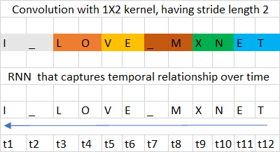
Although feedforward neural networks, including convolution neural networks, have shown great accuracy in classifying sentences and text, they cannot store long-term dependencies in memory (hidden state). Memory can be viewed as temporal state that can updated over time. A feedforward neural network can’t interpret the context since it does not store temporal state (“memory”). A CNN can only learn spatial context from a local group of neighbors (image/sequence) within the size of its convolution kernels. Figure 1 shows the convolution neural network spatial context versus RNN temporal context for a sample data set. In CNN, the relationship between “O” and “V” is lost since they are part of different convolution’s spatial context. In RRN, the temporal relationship between the characters “L”, “O”, “V”, “E” is captured.
It cannot understand learned context since there is no “memory” state. So it cannot model sequential/temporally data (data with definitive ordering, like the structure of a language). An abstract view of a feedforward neural network is shown in Figure 2.
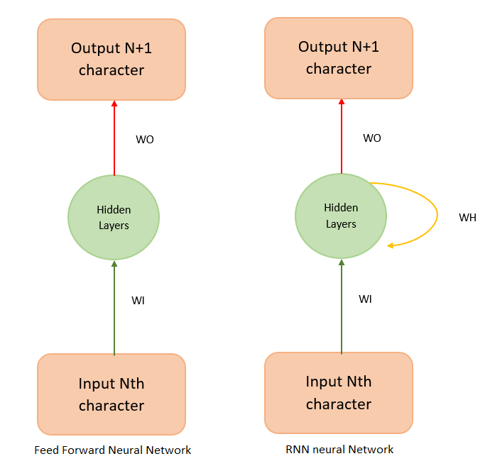
An RNN is more versatile. Its cells accept weighted input and produce both weighted output (WO) and weighted hidden state (WH). The hidden state acts as the memory that stores context. If an RNN represents a person talking on the phone, the weighted output is the words spoken, and the weighted hidden state is the context in which the person utters the word.
The intuition behind RNNs
In this section, we will explain the similarity between a feedforward neural network and RNN by building an unrolled version of a vanilla RNN using a feedforward neural network. A vanilla RNN has a simple hidden state matrix (memory) and is easy to understand and implement.
Suppose we have to predict the 4th character in a stream of text, given the first three characters. To do that, we can design a simple feedforward neural network as in Figure 3.
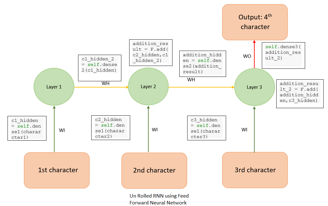
This is basically a feedforward network where the weights WI (green arrows) and WH (yellow arrows) are shared between some of the layers. This is an unrolled version of vanilla RNN, generally referred to as a many-to-one RNN because multiple inputs (three characters, in this case) are used to predict one character. The RNN can be designed using MXNet as follows:
classUnRolledRNN_Model(Block):def__init__(self,vocab_size,num_embed,num_hidden,**kwargs):super(UnRolledRNN_Model,self).__init__(**kwargs)self.num_embed=num_embedself.vocab_size=vocab_size# use name_scope to give child Blocks appropriate names.# It also allows sharing Parameters between Blocks recursively.withself.name_scope():self.encoder=nn.Embedding(self.vocab_size,self.num_embed)self.dense1=nn.Dense(num_hidden,activation='relu',flatten=True)self.dense2=nn.Dense(num_hidden,activation='relu',flatten=True)self.dense3=nn.Dense(vocab_size,flatten=True)defforward(self,inputs):emd=self.encoder(inputs)# print( emd.shape )# since the input is shape (batch_size, input(3 characters) )# we need to extract 0th, 1st, 2nd character from each batchcharacter1=emd[:,0,:]character2=emd[:,1,:]character3=emd[:,2,:]# green arrow in diagram for character 1c1_hidden=self.dense1(character1)# green arrow in diagram for character 2c2_hidden=self.dense1(character2)# green arrow in diagram for character 3c3_hidden=self.dense1(character3)# yellow arrow in diagramc1_hidden_2=self.dense2(c1_hidden)addition_result=F.add(c2_hidden,c1_hidden_2)# Total c1 + c2addition_hidden=self.dense2(addition_result)# the yellow arrowaddition_result_2=F.add(addition_hidden,c3_hidden)# Total c1 + c2final_output=self.dense3(addition_result_2)returnfinal_outputvocab_size=len(chars)+1# the vocabsizenum_embed=30num_hidden=256# model creationsimple_model=UnRolledRNN_Model(vocab_size,num_embed,num_hidden)# model initilisationsimple_model.collect_params().initialize(mx.init.Xavier(),ctx=context)trainer=gluon.Trainer(simple_model.collect_params(),'adam')loss=gluon.loss.SoftmaxCrossEntropyLoss()
Basically, this neural network has embedding layers (emb) followed by three dense layers:
Dense 1 (with weights WI), which accepts the input
Dense 2 (with weights WH) (an intermediate layer)
Dense 3 (with weights WO), which produces the output. We also do some MXNet array addition to combine inputs.
You can check this blog post to learn about the embedding layer and its functionality. The dense layers 1, 2, and 3 learn a set of weights that can predict the 4th character given the first three characters.
We use binary cross entropy loss in our model. This model can be folded back and succinctly represented as in Figure 4.
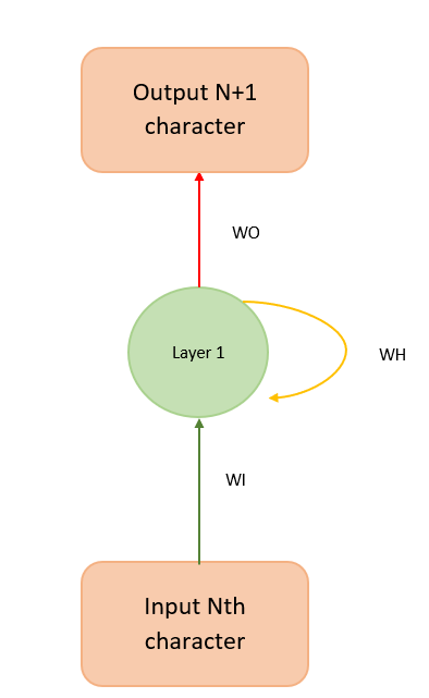
Figure 4 helps explain the math behind the model, which can be carried out as follows:
hidden_state_at_t=tanh(WIxinput+WHxprevious_hidden_state+bias)
Vanilla RNNs have some limitations. For example, let’s say we have a long document containing the sentences, “I was born in France during the world war” and, “So I can speak French.” A vanilla RNN cannot understand the context of being “born in France” and “I can speak French” if they are far apart in a given document.
An RNN doesn’t provide the capability (at least in practice) to forget the irrelevant context in between the phrases. An RNN gives more importance to the most previous hidden state because it cannot give preference to the arbitrary (t-k) hidden state, where t is the current time step and k is a number greater than 0. This is because training an RNN on a long sequence of words can cause the gradient to vanish (when the gradient is small) or to explode (when the gradient is large) during backpropagation.
Basically, the backpropagation algorithm multiplies the gradients along the computational graph of the neural network in reverse direction. Hence, when the eigenvalue of the hidden state matrix is large or small, the gradient becomes unstable. A detailed explanation of the problems with RNN is explained here.
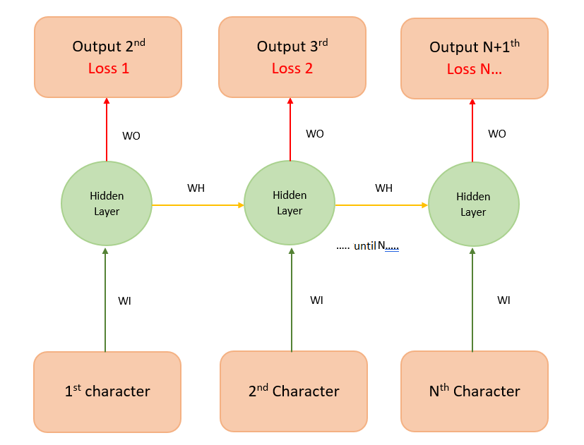
In addition to the many-to-one RNN, there are other types of RNNs that process such memory-based applications, including the popular sequence-to-sequence RNN (see Figure 5). In this sequence-to-sequence RNN, where the sequence length is 3, each input is mapped onto a separate output. This helps the model to train faster because we measure loss (the difference between the predicted value and the actual output) at each time instant. Instead of one loss at the end, we can see loss1, loss2, etc., so that we get better feedback (backpropagation) when training our model.
Long short-term memory (LSTM)
To address the problems with vanilla RNN, two German researchers, Sepp Hochreiter and Juergen Schmidhuber, proposed long short-term memory (LSTM), a complex RNN unit, as a solution to the vanishing/exploding gradient problem. Some beautifully illustrated, simple versions of LSTM can be found here and here. In an abstract sense, we can think of the LSTM unit as a small neural network that decides the amount of information it needs to preserve (memory) from the previous time step.
Implementing an LSTM
Now we can try creating our own simple character predictor.
Preparing your environment
If you’re working in the AWS Cloud, you can save yourself a lot of installation work by using an Amazon SageMaker, pre-configured for deep learning. If you have done this, skip steps 1-5 below.
If you are using a Conda environment, remember to install pip inside conda by typing conda install pip after you activate an environment. This will save you a lot of problems down the road.
Here’s how to get set up:
Install Anaconda, a package manager. It is easier to install Python libraries using Anaconda.
You can use this command
curl -O https://repo.continuum.io/archive/Anaconda3-4.2.0-Linux-x86_64.sh
chmod 777 Anaconda3-4.2.0-Linux-x86_64.sh
./Anaconda3-4.2.0-Linux-x86_64.shInstall scikit-learn, a general-purpose scientific computing library. We’ll use this to pre-process our data. You can install it with
conda install scikit-learn.Grab the Jupyter Notebook, with
conda install jupyter.Get MXNet, an open source deep learning library. The Python notebook was tested on version 0.12.0 of MXNet, and you can install it using pip as follows:
pip install mxnet-cu90(if you have a GPU) otherwise usepip install mxnet --pre. Please see the documentation for details.
- After you activate the anaconda environment, type these commands in it:
source activate mxnet.
The consolidated list of commands is:
curl -O https://repo.continuum.io/archive/Anaconda3-4.2.0-Linux-x86_64.sh

chmod 777 Anaconda3-4.2.0-Linux-x86_64.sh

./Anaconda3-4.2.0-Linux-x86_64.sh

conda install pip

pip install opencv-python

conda install scikit-learn

conda install jupyter

pip install mxnet-cu90
- You can download the MXNet notebook for this part of the tutorial, where we’ve created and run all this code, and play with it! Adjust the hyperparameters and experiment with different approaches to neural network architecture.
Preparing the data set
We will use a work of Friedrich Nietzsche as our data set.
You can download the data set here. You are free to use any other data set, such as your own chat history, or you can download some data sets from this site. If you use your own chat history as the data set, you can write a custom predictive text editor for your own lingo. For now, we will stick with Nietzche’s work.
The data set nietzsche.txt consists of 600,901 characters, out of which 86 are unique. We need to convert the entire text to a sequence of numbers.
# total of characters in datasetchars=sorted(list(set(text)))vocab_size=len(chars)+1('total chars:',vocab_size)# maps character to unique index e.g. {a:1,b:2....}char_indices=dict((c,i)fori,cinenumerate(chars))# maps indices to character (1:a,2:b ....)indices_char=dict((i,c)fori,cinenumerate(chars))# mapping the dataset into indexidx=[char_indices[c]forcintext]
Preparing the data set for an unrolled RNN
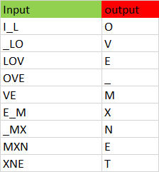
Our goal is to convert the data set to a series of inputs and outputs. Each sequence of three characters from the input stream will be stored as the three input characters to our model, with the next character being the output we are trying to train our model to predict. For instance, we would translate the string I_love_mxnet into the inputs and outputs shown in Figure 6.
The code to do the conversion follows.
# input for neural network(our basic rnn has 3 inputs, n samples)cs=3c1_dat=[idx[i]foriinrange(0,len(idx)-1-cs,cs)]c2_dat=[idx[i+1]foriinrange(0,len(idx)-1-cs,cs)]c3_dat=[idx[i+2]foriinrange(0,len(idx)-1-cs,cs)]# the output of rnn network (single vector)c4_dat=[idx[i+3]foriinrange(0,len(idx)-1-cs,cs)]# stacking the inputs to form (3 input features )x1=np.stack(c1_dat[:-2])x2=np.stack(c2_dat[:-2])x3=np.stack(c3_dat[:-2])# the output (1 X N data points)y=np.stack(c4_dat[:-2])col_concat=np.array([x1,x2,x3])t_col_concat=col_concat.T(t_col_concat.shape)
We also batchify the training set in batches of 32, so that each training instance is of shape 32 X 3. Batchifying the input helps us train the model faster.
# Set the batchsize as 32, so input is of form 32 X 3# output is 32 X 1batch_size=32defget_batch(source,label_data,i,batch_size=32):bb_size=min(batch_size,source.shape[0]-1-i)data=source[i:i+bb_size]target=label_data[i:i+bb_size]# print(target.shape)returndata,target.reshape((-1,))
Preparing the data set for a Gluon RNN
In the previous section, we prepared the data set to predict the 4th character in input, given the previous three characters. In this section, we will generalize the algorithm to predict the nth character, given a sequence with arbitrary length of n-1. This is very similar to preparing the data set for an unrolled RNN, except for the shape of the input. The data set should be ordered in the shape (number of example X batch_size). Now, let us divide the sample data set into batches as shown in Figure 7.
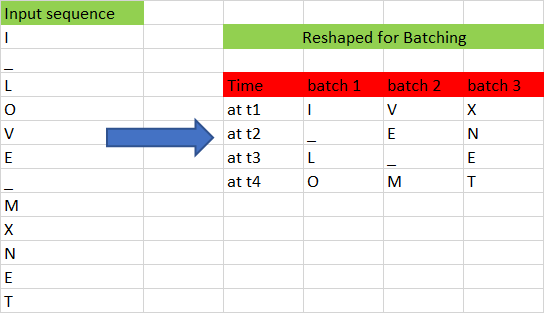
We have converted the input sequence to a batch size of 3 and a sequence length of 4. By transforming it this way, we lose the temporal relationship between many adjacent characters, such as “O” and “V” or “M” and “X”. For example, “V” follows “O” in the input sequence, but “V” and “O” belong to different batches; the only reason we batch the input sequence is to train our model faster. The following Python function does the batching of input:
# prepares rnn batches# The batch will be of shape is (num_example * batch_size) because of RNN uses sequences of input x# for example if we use (a1,a2,a3) as one input sequence , (b1,b2,b3) as another input sequence and (c1,c2,c3)# if we have batch of 3, then at timestep '1' we only have (a1,b1.c1) as input, at timestep '2' we have (a2,b2,c2) as input...# hence the batchsize is of order# In feedforward we use (batch_size, num_example)defrnn_batch(data,batch_size):"""Reshape data into (num_example, batch_size)"""nbatch=data.shape[0]//batch_sizedata=data[:nbatch*batch_size]data=data.reshape((batch_size,nbatch)).Treturndata
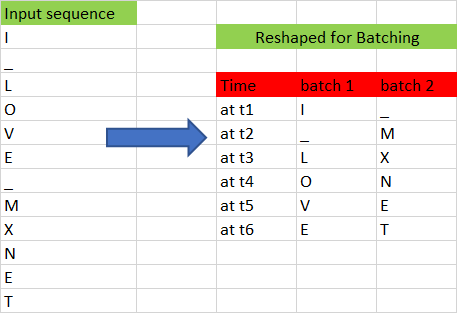
Figure 8 shows another example with batch size 2 and sequence length of 6.
It is very easy to generate an input sequence of arbitrary length from a given batch. For example, if we want to generate a sequence of length 3 from a batch size of 2, we can do so easily using the following code.
#get the batchdefget_batch(source,i,seq):seq_len=min(seq,source.shape[0]-1-i)data=source[i:i+seq_len]target=source[i+1:i+1+seq_len]returndata,target.reshape((-1,))
During our training, we define an input sequence length of 100 as a hyperparameter. This may require fine tuning for the best output.
Designing RNN in Gluon
Next, we define a class that allows us to create two RNN models that we have chosen for our example: GRU (gated recurrent unit) and LSTM. GRU is a simpler version of LSTM and performs equally well. You can find a comparison study here. The models are created with the following Python snippet:
classGluonRNNModel(gluon.Block):"""A model with an encoder, recurrent layer, and a decoder."""def__init__(self,mode,vocab_size,num_embed,num_hidden,num_layers,dropout=0.5,**kwargs):super(GluonRNNModel,self).__init__(**kwargs)withself.name_scope():self.drop=nn.Dropout(dropout)self.encoder=nn.Embedding(vocab_size,num_embed,weight_initializer=mx.init.Uniform(0.1))ifmode=='lstm':# we create a LSTM layer with certain number of hidden LSTM cell and layers# in our example num_hidden is 1000 and num of layers is 2# The input to the LSTM will only be passed during the forward pass (see forward function below)self.rnn=rnn.LSTM(num_hidden,num_layers,dropout=dropout,input_size=num_embed)elifmode=='gru':# we create a GRU layer with certain number of hidden GRU cell and layers# in our example num_hidden is 1000 and num of layers is 2# The input to the GRU will only be passed during the forward pass (see forward function below)self.rnn=rnn.GRU(num_hidden,num_layers,dropout=dropout,input_size=num_embed)else:# we create a vanilla RNN layer with certain number of hidden vanilla RNN cell and layers# in our example num_hidden is 1000 and num of layers is 2# The input to the vanilla will only be passed during the forward pass (see forward function below)self.rnn=rnn.RNN(num_hidden,num_layers,activation='relu',dropout=dropout,input_size=num_embed)self.decoder=nn.Dense(vocab_size,in_units=num_hidden)self.num_hidden=num_hidden# define the forward pass of the neural networkdefforward(self,inputs,hidden):emb=self.encoder(inputs)# emb, hidden are the inputs to the hiddenoutput,hidden=self.rnn(emb,hidden)# the ouput from the hidden layer to passed to drop out layeroutput=self.drop(output)# print('output forward',output.shape)# Then the output is flattened to a shape for the dense layerdecoded=self.decoder(output.reshape((-1,self.num_hidden)))returndecoded,hidden# Initial state of RNN layerdefbegin_state(self,*args,**kwargs):returnself.rnn.begin_state(*args,**kwargs)
The constructor of the class creates the neural units that will be used in our forward pass. The constructor is parameterized by the type of RNN layer to use: LSTM, GRU, or vanilla RNN. The forward pass method will be called when training the model to generate the loss associated with the training data.
The forward pass function starts by creating an embedding layer for the input character. You can look at our previous blog post for more details on embedding. The output of the embedding layer is provided as input to the RNN. The RNN returns an output as well as the hidden state. A dropout layer keeps the model from memorizing the input-output mapping, to prevent overfitting. The output produced by the RNN is passed to a decoder (dense unit), which predicts the next character in the neural network and also generates the loss during the training phase.
We also have a “begin state” function that initializes the initial hidden state of the model.
Training the neural network
After defining the network, now, we have to train the neural network so that it learns.
deftrainGluonRNN(epochs,train_data,seq=seq_length):forepochinrange(epochs):total_L=0.0hidden=model.begin_state(func=mx.nd.zeros,batch_size=batch_size,ctx=context)foribatch,iinenumerate(range(0,train_data.shape[0]-1,seq_length)):data,target=get_batch(train_data,i,seq)hidden=detach(hidden)withautograd.record():output,hidden=model(data,hidden)L=loss(output,target)# this is total loss associated with seq_lengthL.backward()grads=[i.grad(context)foriinmodel.collect_params().values()]# Here gradient is for the whole batch.# So we multiply max_norm by batch_size and seq_length to balance it.gluon.utils.clip_global_norm(grads,clip*seq_length*batch_size)trainer.step(batch_size)total_L+=mx.nd.sum(L).asscalar()ifibatch%log_interval==0andibatch>0:cur_L=total_L/seq_length/batch_size/log_interval('[Epoch%dBatch%d] loss%.2f',epoch+1,ibatch,cur_L)total_L=0.0model.save_params(rnn_save)
Each epoch starts by initializing the hidden units to zero. While training each batch, we detach the hidden unit from computational graph so that we don’t backpropagate the gradient beyond the sequence length (100 in our case). If we don’t detach the hidden state, the gradient is passed to the beginning of hidden state (t=0). After detaching, we calculate the loss and use the backward function to backpropagate the loss in order to fine tune the weights. We also normalize the gradient by multiplying it by the sequence length and batch size.
Text generation
Once the model is trained with the input data, we can generate random text similar to the input data. The weights of the trained model (200 epochs) with sequence length of 100 is available here. You can download the model weights and load it using the model.load_params function.
Next, we will use this model to generate text similar to the text in the “nietzsche” input. To generate a sequence of arbitrary length, we use the output generated by the model as the input for the next iteration.
To generate text, we initialize the hidden state.
hidden=model.begin_state(func=mx.nd.zeros,batch_size=batch_size,ctx=context)
Remember, we don’t have to reset the hidden state because we don’t backpropagate the loss to fine tune the weights.
Then, we reshape the input sequence vector to a shape that the RNN model accepts.
sample_input=mx.nd.array(np.array([idx[0:seq_length]]).T,ctx=context)
Then we look at the argmax of the output produced by the network. generate output char “c”.
output,hidden=model(sample_input,hidden)index=mx.nd.argmax(output,axis=1)index=index.asnumpy()count=count+1
Then append output char “c” to the input string. Next, slice the first character of the input string.
new_string=new_string+indices_char[index[-1]]input_string=input_string[1:]+indices_char[index[-1]]
Below is the full function that generates “nietzsche” like text of arbitrary length.
importsys# a nietzsche like text generatordefgenerate_random_text(model,input_string,seq_length,batch_size,sentence_length):count=0new_string=''cp_input_string=input_stringhidden=model.begin_state(func=mx.nd.zeros,batch_size=batch_size,ctx=context)whilecount<sentence_length:idx=[char_indices[c]forcininput_string]if(len(input_string)!=seq_length):(len(input_string))raiseValueError('there was a error in the input ')sample_input=mx.nd.array(np.array([idx[0:seq_length]]).T,ctx=context)output,hidden=model(sample_input,hidden)index=mx.nd.argmax(output,axis=1)index=index.asnumpy()count=count+1new_string=new_string+indices_char[index[-1]]input_string=input_string[1:]+indices_char[index[-1]](cp_input_string+new_string)
If you look at the text generated, you’ll notice that the model has learned open and close quotations(“”). It has a definite structure and looks similar to “nietzsche”.
You can also train a model on your chat history to predict the next character you will type.
In our next article, we will take a look at generative models*, especially generative adversarial networks, a powerful model that can generate new data from a given input data set.
This post is a collaboration between O’Reilly and Amazon. See our statement of editorial independence.