Hadoop with Python
Learn how to use Python with the Hadoop Distributed File System, MapReduce, the Apache Pig platform and Pig Latin script, and the Apache Spark cluster-computing framework.
 Elephant and python (source: O'Reilly)
Source Code
All of the source code in this book is on GitHub. To copy the source code locally, use the following git clone command:
$ git clone https://github.com/MinerKasch/HadoopWithPython
Hadoop Distributed File System (HDFS)
The Hadoop Distributed File System (HDFS) is a Java-based distributed, scalable, and portable filesystem designed to span large clusters of commodity servers. The design of HDFS is based on GFS, the Google File System, which is described in a paper published by Google. Like many other distributed filesystems, HDFS holds a large amount of data and provides transparent access to many clients distributed across a network. Where HDFS excels is in its ability to store very large files in a reliable and scalable manner.

Learn faster. Dig deeper. See farther.
HDFS is designed to store a lot of information, typically petabytes (for very large files), gigabytes, and terabytes. This is accomplished by using a block-structured filesystem. Individual files are split into fixed-size blocks that are stored on machines across the cluster. Files made of several blocks generally do not have all of their blocks stored on a single machine.
HDFS ensures reliability by replicating blocks and distributing the replicas across the cluster. The default replication factor is three, meaning that each block exists three times on the cluster. Block-level replication enables data availability even when machines fail.
This chapter begins by introducing the core concepts of HDFS and explains how to interact with the filesystem using the native built-in commands. After a few examples, a Python client library is introduced that enables HDFS to be accessed programmatically from within Python applications.
Overview of HDFS
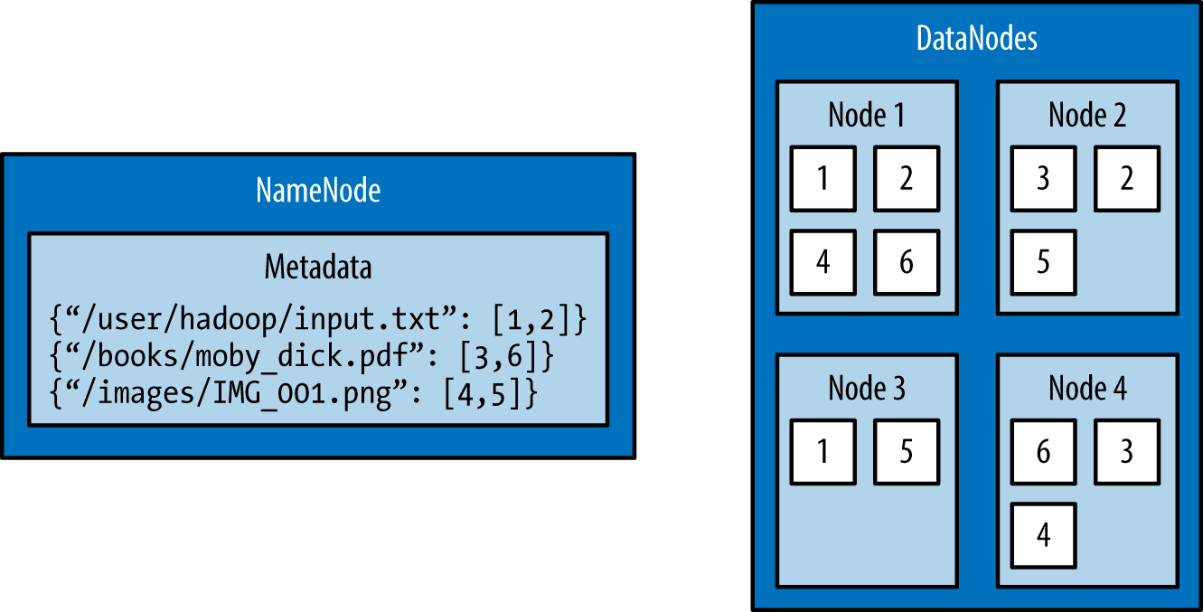
The architectural design of HDFS is composed of two processes: a process known as the NameNode holds the metadata for the filesystem, and one or more DataNode processes store the blocks that make up the files. The NameNode and DataNode processes can run on a single machine, but HDFS clusters commonly consist of a dedicated server running the NameNode process and possibly thousands of machines running the DataNode process.
The NameNode is the most important machine in HDFS. It stores metadata for the entire filesystem: filenames, file permissions, and the location of each block of each file. To allow fast access to this information, the NameNode stores the entire metadata structure in memory. The NameNode also tracks the replication factor of blocks, ensuring that machine failures do not result in data loss. Because the NameNode is a single point of failure, a secondary NameNode can be used to generate snapshots of the primary NameNode’s memory structures, thereby reducing the risk of data loss if the NameNode fails.
The machines that store the blocks within HDFS are referred to as DataNodes. DataNodes are typically commodity machines with large storage capacities. Unlike the NameNode, HDFS will continue to operate normally if a DataNode fails. When a DataNode fails, the NameNode will replicate the lost blocks to ensure each block meets the minimum replication factor.
The example in Figure 1-1 illustrates the mapping of files to blocks in the NameNode, and the storage of blocks and their replicas within the DataNodes.
The following section describes how to interact with HDFS using the built-in commands.
Interacting with HDFS
Interacting with HDFS is primarily performed from the command line using the script named hdfs. The hdfs script has the following usage:
$ hdfs COMMAND [-option <arg>]
The COMMAND argument instructs which functionality of HDFS will be used. The -option argument is the name of a specific option for the specified command, and <arg> is one or more arguments that that are specified for this option.
Common File Operations
To perform basic file manipulation operations on HDFS, use the dfs command with the hdfs script. The dfs command supports many of the same file operations found in the Linux shell.
It is important to note that the hdfs command runs with the permissions of the system user running the command. The following examples are run from a user named “hduser.”
List Directory Contents
To list the contents of a directory in HDFS, use the -ls command:
$ hdfs dfs -ls
$
Running the -ls command on a new cluster will not return any results. This is because the -ls command, without any arguments, will attempt to display the contents of the user’s home directory on HDFS. This is not the same home directory on the host machine (e.g., /home/$USER), but is a directory within HDFS.
Providing -ls with the forward slash (/) as an argument displays the contents of the root of HDFS:
$ hdfs dfs -ls /
Found 2 items
drwxr-xr-x   - hadoop supergroup    0 2015-09-20 14:36 /hadoop
drwx------   - hadoop supergroup    0 2015-09-20 14:36 /tmp
The output provided by the hdfs dfs command is similar to the output on a Unix filesystem. By default, -ls displays the file and folder permissions, owners, and groups. The two folders displayed in this example are automatically created when HDFS is formatted. The hadoop user is the name of the user under which the Hadoop daemons were started (e.g., NameNode and DataNode), and the supergroup is the name of the group of superusers in HDFS (e.g., hadoop).
Creating a Directory
Home directories within HDFS are stored in /user/$HOME. From the previous example with -ls, it can be seen that the /user directory does not currently exist. To create the /user directory within HDFS, use the -mkdir command:
$ hdfs dfs -mkdir /user
To make a home directory for the current user, hduser, use the -mkdir command again:
$ hdfs dfs -mkdir /user/hduser
Use the -ls command to verify that the previous directories were created:
$ hdfs dfs -ls -R /user
drwxr-xr-x   - hduser supergroup    0 2015-09-22 18:01 /user/hduser
Copy Data onto HDFS
After a directory has been created for the current user, data can be uploaded to the user’s HDFS home directory with the -put command:
$ hdfs dfs -put /home/hduser/input.txt /user/hduser
This command copies the file /home/hduser/input.txt from the local filesystem to /user/hduser/input.txt on HDFS.
Use the -ls command to verify that input.txt was moved to HDFS:
$ hdfs dfs -ls
Found 1 items
-rw-r--r--   1 hduser supergroup         52 2015-09-20 13:20 input.txt
Retrieving Data from HDFS
Multiple commands allow data to be retrieved from HDFS. To simply view the contents of a file, use the -cat command. -cat reads a file on HDFS and displays its contents to stdout. The following command uses -cat to display the contents of /user/hduser/input.txt:
$ hdfs dfs -cat input.txt
jack be nimble
jack be quick
jack jumped over the candlestick
Data can also be copied from HDFS to the local filesystem using the -get command. The -get command is the opposite of the -put command:
$ hdfs dfs -get input.txt /home/hduser
This command copies input.txt from /user/hduser on HDFS to /home/hduser on the local filesystem.
HDFS Command Reference
The commands demonstrated in this section are the basic file operations needed to begin using HDFS. Below is a full listing of file manipulation commands possible with hdfs dfs. This listing can also be displayed from the command line by specifying hdfs dfs without any arguments. To get help with a specific option, use either hdfs dfs -usage <option> or hdfs dfs -help <option>.
Usage: hadoop fs [generic options]
    [-appendToFile <localsrc> ... <dst>]
    [-cat [-ignoreCrc] <src> ...]
    [-checksum <src> ...]
    [-chgrp [-R] GROUP PATH...]
    [-chmod [-R] <MODE[,MODE]... | OCTALMODE> PATH...]
    [-chown [-R] [OWNER][:[GROUP]] PATH...]
    [-copyFromLocal [-f] [-p] [-l] <localsrc> ... <dst>]
    [-copyToLocal [-p] [-ignoreCrc] [-crc] <src> ... <localdst>]
    [-count [-q] [-h] <path> ...]
    [-cp [-f] [-p | -p[topax]] <src> ... <dst>]
    [-createSnapshot <snapshotDir> [<snapshotName>]]
    [-deleteSnapshot <snapshotDir> <snapshotName>]
    [-df [-h] [<path> ...]]
    [-du [-s] [-h] <path> ...]
    [-expunge]
    [-find <path> ... <expression> ...]
    [-get [-p] [-ignoreCrc] [-crc] <src> ... <localdst>]
    [-getfacl [-R] <path>]
    [-getfattr [-R] {-n name | -d} [-e en] <path>]
    [-getmerge [-nl] <src> <localdst>]
    [-help [cmd ...]]
    [-ls [-d] [-h] [-R] [<path> ...]]
    [-mkdir [-p] <path> ...]
    [-moveFromLocal <localsrc> ... <dst>]
    [-moveToLocal <src> <localdst>]
    [-mv <src> ... <dst>]
    [-put [-f] [-p] [-l] <localsrc> ... <dst>]
    [-renameSnapshot <snapshotDir> <oldName> <newName>]
    [-rm [-f] [-r|-R] [-skipTrash] <src> ...]
    [-rmdir [--ignore-fail-on-non-empty] <dir> ...]
    [-setfacl [-R] [{-b|-k} {-m|-x <acl_spec>} <path>]|[--set <acl_spec> <path>]]
    [-setfattr {-n name [-v value] | -x name} <path>]
    [-setrep [-R] [-w] <rep> <path> ...]
    [-stat [format] <path> ...]
    [-tail [-f] <file>]
    [-test -[defsz] <path>]
    [-text [-ignoreCrc] <src> ...]
    [-touchz <path> ...]
    [-truncate [-w] <length> <path> ...]
    [-usage [cmd ...]]

Generic options supported are
-conf <configuration file>     specify an application configuration file
-D <property=value>            use value for given property
-fs <local|namenode:port>      specify a namenode
-jt <local|resourcemanager:port>    specify a ResourceManager
-files <comma separated list of files>    specify comma separated files to be copied to the map reduce cluster
-libjars <comma separated list of jars>    specify comma separated jar files to include in the classpath.
-archives <comma separated list of archives>    specify comma separated archives to be unarchived on the compute machines.

The general command line syntax is
bin/hadoop command [genericOptions] [commandOptions]
The next section introduces a Python library that allows HDFS to be accessed from within Python applications.
Snakebite
Snakebite is a Python package, created by Spotify, that provides a Python client library, allowing HDFS to be accessed programmatically from Python applications. The client library uses protobuf messages to communicate directly with the NameNode. The Snakebite package also includes a command-line interface for HDFS that is based on the client library.
This section describes how to install and configure the Snakebite package. Snakebite’s client library is explained in detail with multiple examples, and Snakebite’s built-in CLI is introduced as a Python alternative to the hdfs dfs command.
Installation
Snakebite requires Python 2 and python-protobuf 2.4.1 or higher. Python 3 is currently not supported.
Snakebite is distributed through PyPI and can be installed using pip:
$ pip install snakebite
Client Library
The client library is written in Python, uses protobuf messages, and implements the Hadoop RPC protocol for talking to the NameNode. This enables Python applications to communicate directly with HDFS and not have to make a system call to hdfs dfs.
List Directory Contents
Example 1-1 uses the Snakebite client library to list the contents of the root directory in HDFS.
Example 1-1. python/HDFS/list_directory.py
from snakebite.client import Client

client = Client('localhost', 9000)
for x in client.ls(['/']):
   print x
The most important line of this program, and every program that uses the client library, is the line that creates a client connection to the HDFS NameNode:
client = Client('localhost', 9000)
The Client() method accepts the following parameters:
host (string)- Hostname or IP address of the NameNode
port (int)- RPC port of the NameNode
hadoop_version (int)- The Hadoop protocol version to be used (default: 9)
use_trash (boolean)- Use trash when removing files
effective_use (string)- Effective user for the HDFS operations (default: None or current user)
The host and port parameters are required and their values are dependent upon the HDFS configuration. The values for these parameters can be found in the hadoop/conf/core-site.xml configuration file under the property fs.defaultFS:
<property>
   <name>fs.defaultFS</name>
   <value>hdfs://localhost:9000</value>
</property>
For the examples in this section, the values used for host and port are localhost and 9000, respectively.
After the client connection is created, the HDFS filesystem can be accessed. The remainder of the previous application used the ls command to list the contents of the root directory in HDFS:
for x in client.ls(['/']):
   print x
It is important to note that many of methods in Snakebite return generators. Therefore they must be consumed to execute. The ls method takes a list of paths and returns a list of maps that contain the file information.
Executing the list_directory.py application yields the following results:
$ python list_directory.py
{'group': u'supergroup', 'permission': 448, 'file_type': 'd', 'access_time': 0L, 'block_replication': 0, 'modification_time': 1442752574936L, 'length': 0L, 'blocksize': 0L, 'owner': u'hduser', 'path': '/tmp'}
{'group': u'supergroup', 'permission': 493, 'file_type': 'd', 'access_time': 0L, 'block_replication': 0, 'modification_time': 1442742056276L, 'length': 0L, 'blocksize': 0L, 'owner': u'hduser', 'path': '/user'}
Create a Directory
Use the mkdir() method to create directories on HDFS. Example 1-2 creates the directories /foo/bar and /input on HDFS.
Example 1-2. python/HDFS/mkdir.py
from snakebite.client import Client

client = Client('localhost', 9000)
for p in client.mkdir(['/foo/bar', '/input'], create_parent=True):
   print p
Executing the mkdir.py application produces the following results:
$ python mkdir.py
{'path': '/foo/bar', 'result': True}
{'path': '/input', 'result': True}
The mkdir() method takes a list of paths and creates the specified paths in HDFS. This example used the create_parent parameter to ensure that parent directories were created if they did not already exist. Setting create_parent to True is analogous to the mkdir -p Unix command.
Deleting Files and Directories
Deleting files and directories from HDFS can be accomplished with the delete() method. Example 1-3 recursively deletes the /foo and /bar directories, created in the previous example.
Example 1-3. python/HDFS/delete.py
from snakebite.client import Client

client = Client('localhost', 9000)
for p in client.delete(['/foo', '/input'], recurse=True):
   print p
Executing the delete.py application produces the following results:
$ python delete.py
{'path': '/foo', 'result': True}
{'path': '/input', 'result': True}
Performing a recursive delete will delete any subdirectories and files that a directory contains. If a specified path cannot be found, the delete method throws a FileNotFoundException. If recurse is not specified and a subdirectory or file exists, DirectoryException is thrown.
The recurse parameter is equivalent to rm -rf and should be used with care.
Retrieving Data from HDFS
Like the hdfs dfs command, the client library contains multiple methods that allow data to be retrieved from HDFS. To copy files from HDFS to the local filesystem, use the copyToLocal() method. Example 1-4 copies the file /input/input.txt from HDFS and places it under the /tmp directory on the local filesystem.
Example 1-4. python/HDFS/copy_to_local.py
from snakebite.client import Client

client = Client('localhost', 9000)
for f in client.copyToLocal(['/input/input.txt'], '/tmp'):
   print f
Executing the copy_to_local.py application produces the following result:
$ python copy_to_local.py
{'path': '/tmp/input.txt', 'source_path': '/input/input.txt', 'result': True, 'error': ''}
To simply read the contents of a file that resides on HDFS, the text() method can be used. Example 1-5 displays the content of /input/input.txt.
Example 1-5. python/HDFS/text.py
from snakebite.client import Client

client = Client('localhost', 9000)
for l in client.text(['/input/input.txt']):
   print l
Executing the text.py application produces the following results:
$ python text.py
jack be nimble
jack be quick
jack jumped over the candlestick
The text() method will automatically uncompress and display gzip and bzip2 files.
CLI Client
The CLI client included with Snakebite is a Python command-line HDFS client based on the client library. To execute the Snakebite CLI, the hostname or IP address of the NameNode and RPC port of the NameNode must be specified. While there are many ways to specify these values, the easiest is to create a ~.snakebiterc configuration file. Example 1-6 contains a sample config with the NameNode hostname of localhost and RPC port of 9000.
Example 1-6. ~/.snakebiterc
{
    "config_version": 2,
    "skiptrash": true,
    "namenodes": [
        {"host": "localhost", "port": 9000, "version": 9},
    ]
}
The values for host and port can be found in the hadoop/conf/core-site.xml configuration file under the property fs.defaultFS.
For more information on configuring the CLI, see the Snakebite CLI documentation online.
Usage
To use the Snakebite CLI client from the command line, simply use the command snakebite. Use the ls option to display the contents of a directory:
$ snakebite ls /
Found 2 items
drwx------   - hadoop    supergroup    0 2015-09-20 14:36 /tmp
drwxr-xr-x   - hadoop    supergroup    0 2015-09-20 11:40 /user
Like the hdfs dfs command, the CLI client supports many familiar file manipulation commands (e.g., ls, mkdir, df, du, etc.).
The major difference between snakebite and hdfs dfs is that snakebite is a pure Python client and does not need to load any Java libraries to communicate with HDFS. This results in quicker interactions with HDFS from the command line.
CLI Command Reference
The following is a full listing of file manipulation commands possible with the snakebite CLI client. This listing can be displayed from the command line by specifying snakebite without any arguments. To view help with a specific command, use snakebite [cmd] --help, where cmd is a valid snakebite command.
snakebite [general options] cmd [arguments]
general options:
  -D --debug               Show debug information
  -V --version             Hadoop protocol version (default:9)
  -h --help                show help
  -j --json                JSON output
  -n --namenode            namenode host
  -p --port                namenode RPC port (default: 8020)
  -v --ver                 Display snakebite version

commands:
  cat [paths]                  copy source paths to stdout
  chgrp <grp> [paths]          change group
  chmod <mode> [paths]         change file mode (octal)
  chown <owner:grp> [paths]    change owner
  copyToLocal [paths] dst      copy paths to local
                                 file system destination
  count [paths]                display stats for paths
  df                           display fs stats
  du [paths]                   display disk usage statistics
  get file dst                 copy files to local
                                 file system destination
  getmerge dir dst             concatenates files in source dir
                                 into destination local file
  ls [paths]                   list a path
  mkdir [paths]                create directories
  mkdirp [paths]               create directories and their
                                 parents
  mv [paths] dst               move paths to destination
  rm [paths]                   remove paths
  rmdir [dirs]                 delete a directory
  serverdefaults               show server information
  setrep <rep> [paths]         set replication factor
  stat [paths]                 stat information
  tail path                    display last kilobyte of the
                                 file to stdout
  test path                    test a path
  text path [paths]            output file in text format
  touchz [paths]               creates a file of zero length
  usage <cmd>                  show cmd usage

to see command-specific options use: snakebite [cmd] --help
Chapter Summary
This chapter introduced and described the core concepts of HDFS. It explained how to interact with the filesystem using the built-in hdfs dfs command. It also introduced the Python library, Snakebite. Snakebite’s client library was explained in detail with multiple examples. The snakebite CLI was also introduced as a Python alternative to the hdfs dfs command.
MapReduce with Python
MapReduce is a programming model that enables large volumes of data to be processed and generated by dividing work into independent tasks and executing the tasks in parallel across a cluster of machines. The MapReduce programming style was inspired by the functional programming constructs map and reduce, which are commonly used to process lists of data. At a high level, every MapReduce program transforms a list of input data elements into a list of output data elements twice, once in the map phase and once in the reduce phase.
This chapter begins by introducing the MapReduce programming model and describing how data flows through the different phases of the model. Examples then show how MapReduce jobs can be written in Python.
Data Flow
The MapReduce framework is composed of three major phases: map, shuffle and sort, and reduce. This section describes each phase in detail.
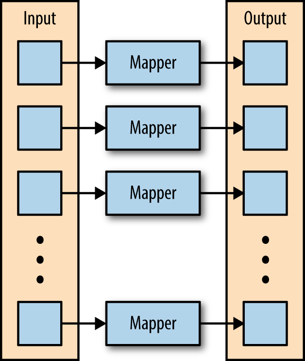
Map
The first phase of a MapReduce application is the map phase. Within the map phase, a function (called the mapper) processes a series of key-value pairs. The mapper sequentially processes each key-value pair individually, producing zero or more output key-value pairs (Figure 2-1).
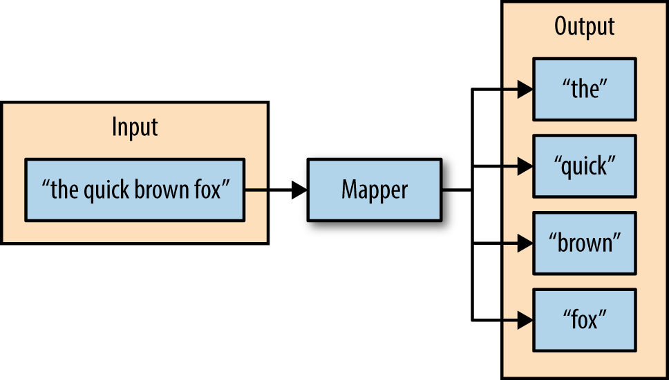
As an example, consider a mapper whose purpose is to transform sentences into words. The input to this mapper would be strings that contain sentences, and the mapper’s function would be to split the sentences into words and output the words (Figure 2-2).
Shuffle and Sort
The second phase of MapReduce is the shuffle and sort. As the mappers begin completing, the intermediate outputs from the map phase are moved to the reducers. This process of moving output from the mappers to the reducers is known as shuffling.
Shuffling is handled by a partition function, known as the partitioner. The partitioner is used to control the flow of key-value pairs from mappers to reducers. The partitioner is given the mapper’s output key and the number of reducers, and returns the index of the intended reducer. The partitioner ensures that all of the values for the same key are sent to the same reducer. The default partitioner is hash-based. It computes a hash value of the mapper’s output key and assigns a partition based on this result.
The final stage before the reducers start processing data is the sorting process. The intermediate keys and values for each partition are sorted by the Hadoop framework before being presented to the reducer.
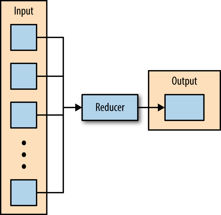
Reduce
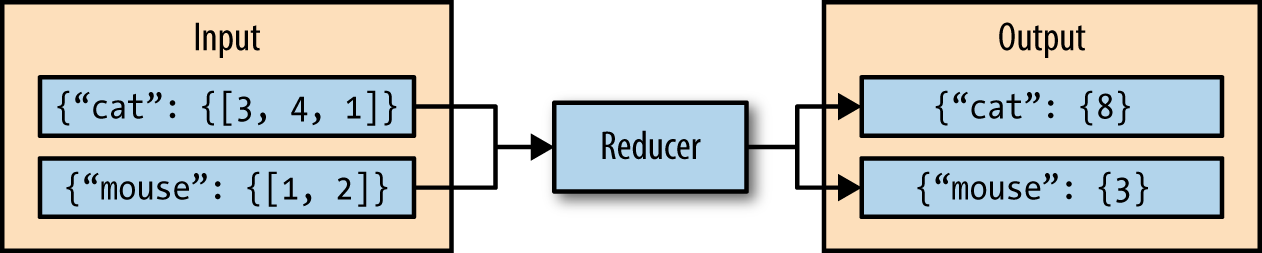
The third phase of MapReduce is the reduce phase. Within the reducer phase, an iterator of values is provided to a function known as the reducer. The iterator of values is a nonunique set of values for each unique key from the output of the map phase. The reducer aggregates the values for each unique key and produces zero or more output key-value pairs (Figure 2-3).
As an example, consider a reducer whose purpose is to sum all of the values for a key. The input to this reducer is an iterator of all of the values for a key, and the reducer sums all of the values. The reducer then outputs a key-value pair that contains the input key and the sum of the input key values (Figure 2-4).
The next section describes a simple MapReduce application and its implementation in Python.
Hadoop Streaming
Hadoop streaming is a utility that comes packaged with the Hadoop distribution and allows MapReduce jobs to be created with any executable as the mapper and/or the reducer. The Hadoop streaming utility enables Python, shell scripts, or any other language to be used as a mapper, reducer, or both.
How It Works
The mapper and reducer are both executables that read input, line by line, from the standard input (stdin), and write output to the standard output (stdout). The Hadoop streaming utility creates a MapReduce job, submits the job to the cluster, and monitors its progress until it is complete.
When the mapper is initialized, each map task launches the specified executable as a separate process. The mapper reads the input file and presents each line to the executable via stdin. After the executable processes each line of input, the mapper collects the output from stdout and converts each line to a key-value pair. The key consists of the part of the line before the first tab character, and the value consists of the part of the line after the first tab character. If a line contains no tab character, the entire line is considered the key and the value is null.
When the reducer is initialized, each reduce task launches the specified executable as a separate process. The reducer converts the input key-value pair to lines that are presented to the executable via stdin. The reducer collects the executables result from stdout and converts each line to a key-value pair. Similar to the mapper, the executable specifies key-value pairs by separating the key and value by a tab character.
A Python Example
To demonstrate how the Hadoop streaming utility can run Python as a MapReduce application on a Hadoop cluster, the WordCount application can be implemented as two Python programs: mapper.py and reducer.py.
mapper.py is the Python program that implements the logic in the map phase of WordCount. It reads data from stdin, splits the lines into words, and outputs each word with its intermediate count to stdout. The code in Example 2-1 implements the logic in mapper.py.
Example 2-1. python/MapReduce/HadoopStreaming/mapper.py
#!/usr/bin/env python

import sys

# Read each line from stdin
for line in sys.stdin:

  # Get the words in each line
  words = line.split()

  # Generate the count for each word
  for word in words:

     # Write the key-value pair to stdout to be processed by
     # the reducer.
     # The key is anything before the first tab character and the
     #value is anything after the first tab character.
     print '{0}\t{1}'.format(word, 1)
reducer.py is the Python program that implements the logic in the reduce phase of WordCount. It reads the results of mapper.py from stdin, sums the occurrences of each word, and writes the result to stdout. The code in Example 2-2 implements the logic in reducer.py.
Example 2-2. python/MapReduce/HadoopStreaming/reducer.py
#!/usr/bin/env python

import sys

curr_word = None
curr_count = 0

# Process each key-value pair from the mapper
for line in sys.stdin:

  # Get the key and value from the current line
  word, count = line.split('\t')

  # Convert the count to an int
  count = int(count)

  # If the current word is the same as the previous word,
  # increment its count, otherwise print the words count
  # to stdout
  if word == curr_word:
     curr_count += count
  else:

     # Write word and its number of occurrences as a key-value
     # pair to stdout
     if curr_word:
        print '{0}\t{1}'.format(curr_word, curr_count)

     curr_word = word
     curr_count = count

# Output the count for the last word
if curr_word == word:
  print '{0}\t{1}'.format(curr_word, curr_count)
Before attempting to execute the code, ensure that the mapper.py and reducer.py files have execution permission. The following command will enable this for both files:
$ chmod a+x mapper.py reducer.py
Also ensure that the first line of each file contains the proper path to Python. This line enables mapper.py and reducer.py to execute as standalone executables. The value #!/usr/bin/env python should work for most systems, but if it does not, replace /usr/bin/env python with the path to the Python executable on your system.
To test the Python programs locally before running them as a MapReduce job, they can be run from within the shell using the echo and sort commands. It is highly recommended to test all programs locally before running them across a Hadoop cluster.
$ echo 'jack be nimble jack be quick' | ./mapper.py
| sort -t 1 | ./reducer.py
be      2
jack    2
nimble  1
quick   1
Once the mapper and reducer programs are executing successfully against tests, they can be run as a MapReduce application using the Hadoop streaming utility. The command to run the Python programs mapper.py and reducer.py on a Hadoop cluster is as follows:
$ $HADOOP_HOME/bin/hadoop jar
  $HADOOP_HOME/mapred/contrib/streaming/hadoop-streaming*.jar \
-files mapper.py,reducer.py \
-mapper mapper.py \
-reducer reducer.py \
-input /user/hduser/input.txt -output /user/hduser/output
The options used with the Hadoop streaming utility are listed in Table 2-1.
| Option | Description |
-files |
A command-separated list of files to be copied to the MapReduce cluster |
-mapper |
The command to be run as the mapper |
-reducer |
The command to be run as the reducer |
-input |
The DFS input path for the Map step |
-output |
The DFS output directory for the Reduce step |
mrjob
mrjob is a Python MapReduce library, created by Yelp, that wraps Hadoop streaming, allowing MapReduce applications to be written in a more Pythonic manner. mrjob enables multistep MapReduce jobs to be written in pure Python. MapReduce jobs written with mrjob can be tested locally, run on a Hadoop cluster, or run in the cloud using Amazon Elastic MapReduce (EMR).
Writing MapReduce applications with mrjob has many benefits:
- mrjob is currently a very actively developed framework with multiple commits every week.
- mrjob has extensive documentation, more than any other framework or library that supports Python on Hadoop.
- mrjob applications can be executed and tested without having Hadoop installed, enabling development and testing before deploying to a Hadoop cluster.
- mrjob allows MapReduce applications to be written in a single class, instead of writing separate programs for the mapper and reducer.
While mrjob is a great solution, it does have its drawbacks. mrjob is simplified, so it doesn’t give the same level of access to Hadoop that other APIs offer. mrjob does not use typedbytes, so other libraries may be faster.
Installation
The installation of mrjob is simple; it can be installed with pip by using the following command:
$ pip install mrjob
Or it can be installed from source (a git clone):
$ python setup.py install
WordCount in mrjob
Example 2-3 uses mrjob to implement the WordCount algorithm.
Example 2-3. python/MapReduce/mrjob/word_count.py
from mrjob.job import MRJob

class MRWordCount(MRJob):

   def mapper(self, _, line):
      for word in line.split():
         yield(word, 1)

   def reducer(self, word, counts):
      yield(word, sum(counts))

if __name__ == '__main__':
   MRWordCount.run()
To run the mrjob locally, the only thing needed is a body of text. To run the job locally and count the frequency of words within a file named input.txt, use the following command:
$ python word_count.py input.txt
The output depends on the contents of the input file, but should look similar to Example 2-4.
Example 2-4. Output from word_count.py
"be"    2
"jack"    2
"nimble"    1
"quick"    1
What Is Happening
The MapReduce job is defined as the class, MRWordCount. Within the mrjob library, the class that inherits from MRJob contains the methods that define the steps of the MapReduce job. The steps within an mrjob application are mapper, combiner, and reducer. The class inheriting MRJob only needs to define one of these steps.
The mapper() method defines the mapper for the MapReduce job. It takes key and value as arguments and yields tuples of (output_key, output_value). In the WordCount example (Example 2-4), the mapper ignored the input key and split the input value to produce words and counts.
The combiner() method defines the combiner for the MapReduce job. The combiner is a process that runs after the mapper and before the reducer. It receives, as input, all of the data emitted by the mapper, and the output of the combiner is sent to the reducer. The combiner’s input is a key, which was yielded by the mapper, and a value, which is a generator that yields all values yielded by one mapper that corresponds to the key. The combiner yields tuples of (output_key, output_value) as output.
The reducer() method defines the reducer for the MapReduce job. It takes a key and an iterator of values as arguments and yields tuples of (output_key, output_value). In Example 2-4, the reducer sums the value for each key, which represents the frequency of words in the input.
The final component of a MapReduce job written with the mrjob library is the two lines at the end of the file:
if __name__ == '__main__':
   MRWordCount.run()
These lines enable the execution of mrjob; without them, the application will not work.
Executing mrjob
Executing a MapReduce application with mrjob is similar to executing any other Python program. The command line must contain the name of the mrjob application and the input file:
$ python mr_job.py input.txt
By default, mrjob writes output to stdout.
Multiple files can be passed to mrjob as inputs by specifying the filenames on the command line:
$ python mr_job.py input1.txt input2.txt input3.txt
mrjob can also handle input via stdin:
$ python mr_job.py < input.txt
By default, mrjob runs locally, allowing code to be developed and debugged before being submitted to a Hadoop cluster.
To change how the job is run, specify the -r/--runner option. Table 2-2 contains a description of the valid choices for the runner options.
-r inline |
(Default) Run in a single Python process |
-r local |
Run locally in a few subprocesses simulating some Hadoop features |
-r hadoop |
Run on a Hadoop cluster |
-r emr |
Run on Amazon Elastic Map Reduce (EMR) |
Using the runner option allows the mrjob program to be run on a Hadoop cluster, with input being specified from HDFS:
$ python mr_job.py -r hadoop hdfs://input/input.txt
mrjob also allows applications to be run on EMR directly from the command line:
$ python mr_job.py -r emr s3://input-bucket/input.txt
Top Salaries
Example 2-5 uses mrjob to compute employee top annual salaries and gross pay. The dataset used is the salary information from the city of Baltimore for 2014.
Example 2-5. python/MapReduce/mrjob/top_salary.py
from mrjob.job import MRJob
from mrjob.step import MRStep
import csv

cols = 'Name,JobTitle,AgencyID,Agency,HireDate,AnnualSalary,GrossPay'.split(',')

class salarymax(MRJob):

    def mapper(self, _, line):
        # Convert each line into a dictionary
        row = dict(zip(cols, [ a.strip() for a in csv.reader([line]).next()]))

        # Yield the salary
        yield 'salary', (float(row['AnnualSalary'][1:]), line)

        # Yield the gross pay
        try:
            yield 'gross', (float(row['GrossPay'][1:]), line)
        except ValueError:
            self.increment_counter('warn', 'missing gross', 1)

    def reducer(self, key, values):
        topten = []

        # For 'salary' and 'gross' compute the top 10
        for p in values:
            topten.append(p)
            topten.sort()
            topten = topten[-10:]

        for p in topten:
            yield key, p

    combiner = reducer

if __name__ == '__main__':
    salarymax.run()
Use the following command to execute the MapReduce job on Hadoop:
$ python top_salary.py -r hadoop hdfs:///user/hduser/input/salaries.csv
Chapter Summary
This chapter introduced the MapReduce programming model and described how data flows through the different phases of the model. Hadoop Streaming and mrjob were then used to highlight how MapReduce jobs can be written in Python.
Pig and Python
Pig is composed of two major parts: a high-level data flow language called Pig Latin, and an engine that parses, optimizes, and executes the Pig Latin scripts as a series of MapReduce jobs that are run on a Hadoop cluster. Compared to Java MapReduce, Pig is easier to write, understand, and maintain because it is a data transformation language that allows the processing of data to be described as a sequence of transformations. Pig is also highly extensible through the use of the User Defined Functions (UDFs) which allow custom processing to be written in many languages, such as Python.
An example of a Pig application is the Extract, Transform, Load (ETL) process that describes how an application extracts data from a data source, transforms the data for querying and analysis purposes, and loads the result onto a target data store. Once Pig loads the data, it can perform projections, iterations, and other transformations. UDFs enable more complex algorithms to be applied during the transformation phase. After the data is done being processed by Pig, it can be stored back in HDFS.
This chapter begins with an example Pig script. Pig and Pig Latin are then introduced and described in detail with examples. The chapter concludes with an explanation of how Pig’s core features can be extended through the use of Python.
WordCount in Pig
Example 3-1 implements the WordCount algorithm in Pig. It assumes that a a data file, input.txt, is loaded in HDFS under /user/hduser/input, and output will be placed in HDFS under /user/hduser/output.
Example 3-1. pig/wordcount.pig
%default INPUT '/user/hduser/input/input.txt';
%default OUTPUT '/user/hduser/output';

-- Load the data from the file system into the relation records
records = LOAD '$INPUT';

-- Split each line of text and eliminate nesting
terms = FOREACH records GENERATE FLATTEN(TOKENIZE((chararray) $0)) AS word;

-- Group similar terms
grouped_terms = GROUP terms BY word;

-- Count the number of tuples in each group
word_counts = FOREACH grouped_terms GENERATE COUNT(terms), group;

-- Store the result
STORE word_counts INTO '$OUTPUT';
To execute the Pig script, simply call Pig from the command line and pass it the name of the script to run:
$ pig wordcount.pig
While the job is running, a lot of text will be printed to the console. Once the job is complete, a success message, similar to the one below, will be displayed:
2015-09-26 14:15:10,030 [main] INFO  org.apache.pig.backend.hadoop.executionengine.mapReduceLayer.MapReduceLauncher - Success!
2015-09-26 14:15:10,049 [main] INFO  org.apache.pig.Main - Pig script completed in 18 seconds and 514 milliseconds (18514 ms)
The results of the wordcount.pig script are displayed in Example 3-2 and can be found in HDFS under /user/hduser/output/pig_wordcount/part-r-00000.
Example 3-2. /user/hduser/output/pig_wordcount/part-r-00000
2    be
1    the
3    jack
1    over
1    quick
1    jumped
1    nimble
1    candlestick
WordCount in Detail
This section describes each Pig Latin statement in the wordcount.pig script.
The first statement loads data from the filesystem and stores it in the relation records:
records = LOAD '/user/hduser/input/input.txt';
The second statement splits each line of text using the TOKENIZE function and eliminates nesting using the FLATTEN operator:
terms = FOREACH records GENERATE FLATTEN(TOKENIZE((chararray)$0)) AS word;
The third statement uses the GROUP operator to group the tuples that have the same field:
grouped_terms = GROUP terms BY word;
The fourth statement iterates over all of the terms in each bag and uses the COUNT function to return the sum:
word_counts = FOREACH grouped_terms GENERATE COUNT(terms), group;
The fifth and final statement stores the results in HDFS:
STORE word_counts INTO '/user/hduser/output/pig_wordcount'
Running Pig
Pig contains multiple modes that can be specified to configure how Pig scripts and Pig statements will be executed.
Execution Modes
Pig has two execution modes: local and MapReduce.
Running Pig in local mode only requires a single machine. Pig will run on the local host and access the local filesystem. To run Pig in local mode, use the -x local flag:
$ pig -x local ...
Running Pig in MapReduce mode requires access to a Hadoop cluster. MapReduce mode executes Pig statements and jobs on the cluster and accesses HDFS. To run Pig in MapReduce mode, simply call Pig from the command line or use the -x mapreduce flag:
$ pig ...
or
$ pig -x mapreduce ...
Interactive Mode
Pig can be run interactively in the Grunt shell. To invoke the Grunt shell, simply call Pig from the command line and specify the desired execution mode. The following example starts the Grunt shell in local mode:
pig -x local
...
grunt>
Once the Grunt shell is initialized, Pig Latin statements can be entered and executed in an interactive manner. Running Pig interactively is a great way to learn Pig.
The following example reads /etc/passwd and displays the usernames from within the Grunt shell:
grunt> A = LOAD '/etc/passwd' using PigStorage(':');
grunt> B = FOREACH A GENERATE $0 as username;
grunt> DUMP B;
Batch Mode
Batch mode allows Pig to execute Pig scripts in local or MapReduce mode.
The Pig Latin statements in Example 3-3 read a file named passwd and use the STORE operator to store the results in a directory called user_id.out. Before executing this script, ensure that /etc/passwd is copied to the current working directory if Pig will be run in local mode, or to HDFS if Pig will be executed in MapReduce mode.
Example 3-3. pig/user_id.pig
A = LOAD 'passwd' using PigStorage(':');
B = FOREACH A GENERATE $0 as username;
STORE B INTO 'user_id.out';
Use the following command to execute the user_id.pig script on the local machine:
$ pig -x local user_id.pig
Pig Latin
This section describes the basic concepts of the Pig Latin language, allowing those new to the language to understand and write basic Pig scripts. For a more comprehensive overview of the language, visit the Pig online documentation.
All of the examples in this section load and process data from the tab-delimited file, resources/students (Example 3-4).
Example 3-4. resources/students
john    21    3.89
sally    19    2.56
alice    22    3.76
doug    19    1.98
susan    26    3.25
Statements
Statements are the basic constructs used to process data in Pig. Each statement is an operator that takes a relation as an input, performs a transformation on that relation, and produces a relation as an output. Statements can span multiple lines, but all statements must end with a semicolon (;).
The general form of each Pig script is as follows:
- A
LOADstatement that reads the data from the filesystem - One or more statements to transform the data
- A
DUMPorSTOREstatement to view or store the results, respectively
Loading Data
The LOAD operator is used to load data from the system into Pig. The format of the LOAD operator is as follows:
LOAD 'data' [USING function] [AS schema];
Where 'data' is the name of the file or directory, in quotes, to be loaded. If a directory name is not specified, all of the files within the directory are loaded.
The USING keyword is optional and is used to specify a function to parse the incoming data. If the USING keyword is omitted, the default loading function, PigStorage, is used. The default delimiter is the tab character ('\t').
The AS keyword allows a schema to be defined for the data being loaded. Schemas enable names and datatypes to be declared for individual fields. The following example defines a schema for the data being loaded from the file input.txt. If no schema is defined, the fields are not named and default to type bytearray.
A = LOAD 'students' AS (name:chararray, age:int);

DUMP A;
(john,21,3.89)
(sally,19,2.56)
(alice,22,3.76)
(doug,19,1.98)
(susan,26,3.25)
Transforming Data
Pig contains many operators that enable complex transforming of data. The most common operators are FILTER, FOREACH, and GROUP.
FILTER
The FILTER operator works on tuples or rows of data. It selects tuples from a relation based on a condition.
The following examples use the relation A that contains student data:
A = LOAD 'students' AS (name:chararray, age:int, gpa:float);

DUMP A;
(john,21,3.89)
(sally,19,2.56)
(alice,22,3.76)
(doug,19,1.98)
(susan,26,3.25)
The following example filters out any students under the age of 20, and stores the results in a relation R:
R = FILTER A BY age >= 20;

DUMP R;
(john,21,3.89)
(alice,22,3.76)
(susan,26,3.25)
Condition statements can use the AND, OR, and NOT operators to create more complex FILTER statements. The following example filters out any students with an age less than 20 or a GPA less than or equal to 3.5, and stores the results in a relation R:
R = FILTER A BY (age >= 20) AND (gpa > 3.5)

DUMP R;
(john,21,3.89)
(alice,22,3.76)
FOREACH
While the FILTER operator works on rows of data, the FOREACH operator works on columns of data and is similar to the SELECT statement in SQL.
The following example uses the asterisk (*) to project all of the fields from relation A onto relation X:
R = FOREACH A GENERATE *;

DUMP R;
(john,21,3.89)
(sally,19,2.56)
(alice,22,3.76)
(doug,19,1.98)
(susan,26,3.25)
The following example uses field names to project the age and gpa columns from relation A onto relation X:
R = FOREACH A GENERATE age, gpa;

DUMP R;
(21,3.89)
(19,2.56)
(22,3.76)
(19,1.98)
(26,3.25)
GROUP
The GROUP operator groups together tuples that have the same group key into one or more relations.
The following example groups the student data by age and stores the result into relation B:
B = GROUP A BY age;

DUMP B;
(19,{(doug,19,1.98),(sally,19,2.56)})
(21,{(john,21,3.89)})
(22,{(alice,22,3.76)})
(26,{(susan,26,3.25)})
The result of a GROUP operation is a relation that has one tuple per group. This tuple has two fields: the first field is named group and is of the type of the grouped key; the second field is a bag that takes the name of the original relation. To clarify the structure of relation B, the DESCRIBE and ILLUSTRATE operations can be used:
DESCRIBE B;
B: {group: int,A: {(name: chararray,age: int,gpa: float)}}

ILLUSTRATE B;
------------------------------------------------------------
| B  | group:int  | A:bag{:tuple(name:chararray,            |
                    age:int,gpa:float)}                     |
-------------------------------------------------------------
|    | 19         | {(sally, 19, 2.56), (doug, 19, 1.98)}   |
-------------------------------------------------------------
Using the FOREACH operator, the fields in the previous relation, B, can be referred to by names group and A:
C = FOREACH B GENERATE group, A.name;

DUMP C;
(19,{(doug),(sally)})
(21,{(john)})
(22,{(alice)})
(26,{(susan)})
Storing Data
The STORE operator is used to execute previous Pig statements and store the results on the filesystem. The format of the STORE operator is as follows:
STORE alias INTO 'directory' [USING function];
Where alias is the name of the relation to store, and 'directory' is the name of the storage directory, in quotes. If the directory already exists, the STORE operation will fail. The output files will be named part-nnnnn and are written to the specified directory.
The USING keyword is optional and is used to specify a function to store the data. If the USING keyword is omitted, the default storage function, PigStorage, is used. The following example specifies the PigStorage function to store a file with pipe-delimited fields:
A = LOAD 'students' AS (name:chararray, age:int, gpa:float);

DUMP A;
(john,21,3.89)
(sally,19,2.56)
(alice,22,3.76)
(doug,19,1.98)
(susan,26,3.25)

STORE A INTO 'output' USING PigStorage('|');

CAT output;
john|21|3.89
sally|19|2.56
alice|22|3.76
doug|19|1.98
susan|26|3.25
The provided Pig Latin statements are great general-purpose computing constructs, but are not capable of expressing complex algorithms. The next section describes how to extend the functionality of Pig with Python.
Extending Pig with Python
Pig provides extensive support for custom processing through User Defined Functions (UDFs). Pig currently supports UDFs in six languages: Java, Jython, Python, JavaScript, Ruby, and Groovy.
When Pig executes, it automatically detects the usage of a UDF. To run Python UDFs, Pig invokes the Python command line and streams data in and out of it.
Registering a UDF
Before a Python UDF can be used in a Pig script, it must be registered so Pig knows where to look when the UDF is called. To register a Python UDF file, use Pig’s REGISTER statement:
REGISTER 'udfs/myudf.py' USING streaming_python AS my_udf;
Once the UDF is registered, it can be called from within the Pig script:
relation = FOREACH data GENERATE my_udf.function(field);
In this example the UDF, referenced as my_udf, contains a function called function.
A Simple Python UDF
A simple Python UDF, located in pig/udfs/my_first_udf.py, that returns the integer value 1 each time it is called, is shown in Example 3-5.
Example 3-5. pig/udfs/my_first_udf.py
from pig_util import outputSchema

@outputSchema('value:int')
def return_one():
   """
   Return the integer value 1
   """
   return 1
Some important things to note in this Python script are the from statement on the first line, and the output decorator, @outputSchema decorator, on the third line. These lines enable the Python UDF to define an alias and datatype for the data being returned from the UDF.
The Pig script in Example 3-6 registers the Python UDF and calls the return_one() function in a FOREACH statement.
Example 3-6. pig/simple_udf.pig
REGISTER 'udfs/my_first_udf.py' USING streaming_python AS pyudfs;

A = LOAD '../resources/input.txt';
B = FOREACH A GENERATE pyudfs.return_one();
DUMP B;
When the Pig script is executed, it will generate an integer value 1 for each line in the input file. Use the following command to execute the script (sample output is shown as well):
$ pig -x local simple_udf.pig
...
(1)
(1)
(1)
String Manipulation
Python UDFs are an easy way of extending Pig’s functionality and an easy way to transform and process data.
The Python UDF in Example 3-7 contains two functions: reverse() and num_chars(). The reverse() function takes in a chararray and returns the chararray in reverse order. The num_chars() function takes in a chararray and returns the number of characters in the chararray.
Example 3-7. pig/udfs/string_funcs.py
from pig_util import outputSchema

@outputSchema('word:chararray')
def reverse(word):
   """
   Return the reverse text of the provided word
   """
   return word[::-1]

@outputSchema('length:int')
def num_chars(word):
   """
   Return the length of the provided word
   """
   return len(word)
The Pig script in Example 3-8 loads a text file and applies the reverse() and num_chars() Python functions to each unique word.
Example 3-8. pig/playing_with_words.pig
REGISTER 'udfs/string_funcs.py' USING streaming_python AS string_udf;

-- Load the data from the file system
records = LOAD '../resources/input.txt';

-- Split each line of text and eliminate nesting
terms = FOREACH records GENERATE FLATTEN(TOKENIZE((chararray) $0)) AS word;

-- Group similar terms
grouped_terms = GROUP terms BY word;

-- Count the number of tuples in each group
unique_terms = FOREACH grouped_terms GENERATE group as word;

-- Calculate the number of characters in each term
term_length = FOREACH unique_terms GENERATE word, string_udf.num_chars(word) as length;

-- Display the terms and their length
DUMP term_length;

-- Reverse each word
reverse_terms = FOREACH unique_terms GENERATE word, string_udf.reverse(word) as reverse_word;

-- Display the terms and the reverse terms
DUMP reverse_terms;
Use the following command to execute the script (sample output shown):
$ pig -x local playing_with_words.pig
...
(be,2)
(the,3)
(jack,4)
(over,4)
(quick,5)
(jumped,6)
(nimble,6)
(candlestick,11)
...
(be,eb)
(the,eht)
(jack,kcaj)
(over,revo)
(quick,kciuq)
(jumped,depmuj)
(nimble,elbmin)
(candlestick,kcitseldnac)
Most Recent Movies
The following example uses movie data from the groupLens datasets and external libraries to calculate the 10 most recent movies.
The Python UDF in Example 3-9 contains two functions: parse_title() and days_since_release(). The parse_title() function uses Python’s regular expression module to remove the release year from a movie’s title. The days_since_release() function uses the datetime module to calculate the number of days between the current day and a movie’s release date.
Example 3-9. pig/udfs/movies_udf.py
from pig_util import outputSchema
from datetime import datetime
import re


@outputSchema('title:chararray')
def parse_title(title):
   """
   Return the title without the year
   """
   return re.sub(r'\s*\(\d{4}\)','', title)

@outputSchema('days_since_release:int')
def days_since_release(date):
   """
   Calculate the number of days since the titles release
   """
   if date is None:
      return None

   today = datetime.today()
   release_date = datetime.strptime(date, '%d-%b-%Y')
   delta = today - release_date
   return delta.days
The Pig script in Example 3-10 uses the Python UDFs to determine the 10 most recent movies.
Example 3-10. pig/recent_movies.pig
REGISTER 'udfs/movies_udf.py' USING streaming_python AS movies_udf;

-- Load the data from the file system
records = LOAD '../resources/movies' USING PigStorage('|')
   AS (id:int, title:chararray, release_date:chararray);

-- Parse the titles and determine how many days since the release date
titles = FOREACH records GENERATE movies_udf.parse_title(title), movies_udf.days_since_release(release_date);

-- Order the movies by the time since release
most_recent = ORDER titles BY days_since_release ASC;

-- Get the ten most recent movies
top_ten = LIMIT most_recent 10;

-- Display the top ten most recent movies
DUMP top_ten;
The following command is used to execute the script (sample output shown):
$ pig -x local recent_movies.pig
...
(unknown,)
(Apt Pupil,6183)
(Mighty, The,6197)
(City of Angels,6386)
(Big One, The,6393)
(Lost in Space,6393)
(Mercury Rising,6393)
(Spanish Prisoner, The,6393)
(Hana-bi,6400)
(Object of My Affection, The,6400)
Chapter Summary
This chapter introduced and Pig and Pig Latin. It described the basic concepts of Pig Latin, allowing simple Pig scripts to be created and executed. It also introduced how to extend the functionality of Pig Latin with Python UDFs.
Spark with Python
Spark is a cluster computing framework that uses in-memory primitives to enable programs to run up to a hundred times faster than Hadoop MapReduce applications. Spark applications consist of a driver program that controls the execution of parallel operations across a cluster. The main programming abstraction provided by Spark is known as Resilient Distributed Datasets (RDDs). RDDs are collections of elements partitioned across the nodes of the cluster that can be operated on in parallel.
Spark was created to run on many platforms and be developed in many languages. Currently, Spark can run on Hadoop 1.0, Hadoop 2.0, Apache Mesos, or a standalone Spark cluster. Spark also natively supports Scala, Java, Python, and R. In addition to these features, Spark can be used interactively from a command-line shell.
This chapter begins with an example Spark script. PySpark is then introduced, and RDDs are described in detail with examples. The chapter concludes with example Spark programs written in Python.
WordCount in PySpark
The code in Example 4-1 implements the WordCount algorithm in PySpark. It assumes that a data file, input.txt, is loaded in HDFS under /user/hduser/input, and the output will be placed in HDFS under /user/hduser/output.
Example 4-1. python/Spark/word_count.py
from pyspark import SparkContext

def main():

   sc = SparkContext(appName='SparkWordCount')

   input_file = sc.textFile('/user/hduser/input/input.txt')
   counts = input_file.flatMap(lambda line: line.split()) \
                     .map(lambda word: (word, 1)) \
                     .reduceByKey(lambda a, b: a + b)
   counts.saveAsTextFile('/user/hduser/output')

   sc.stop()

if __name__ == '__main__':
   main()
To execute the Spark application, pass the name of the file to the spark-submit script:
$ spark-submit --master local word_count.py
While the job is running, a lot of text will be printed to the console. The results of a word_count.py Spark script are displayed in Example 4-2 and can be found in HDFS under /user/hduser/output/part-00000.
Example 4-2. /user/hduser/output/part-00000
(u'be', 2)
(u'jumped', 1)
(u'over', 1)
(u'candlestick', 1)
(u'nimble', 1)
(u'jack', 3)
(u'quick', 1)
(u'the', 1)
WordCount Described
This section describes the transformations being applied in the word_count.py Spark script.
The first statement creates a SparkContext object. This object tells Spark how and where to access a cluster:
sc = SparkContext(appName='SparkWordCount')
The second statement uses the SparkContext to load a file from HDFS and store it in the variable input_file:
input_file = sc.textFile('/user/hduser/input/input.txt')
The third statement performs multiple transformations on the input data. Spark automatically parallelizes these transformations to run across multiple machines:
counts = input_file.flatMap(lambda line: line.split()) \
                   .map(lambda word: (word, 1)) \
                   .reduceByKey(lambda a, b: a + b)
The fourth statement stores the results to HDFS:
counts.saveAsTextFile('/user/hduser/output')
The fifth statement shuts down the SparkContext:
sc.stop()
PySpark
PySpark is Spark’s Python API. PySpark allows Spark applications to be created from an interactive shell or from Python programs.
Before executing any code within Spark, the application must create a SparkContext object. The SparkContext object tells Spark how and where to access a cluster. The master property is a cluster URL that determines where the Spark appliction will run. The most common values for master are:
local- Run Spark with one worker thread.
local[n]- Run Spark with
nworker threads. spark://HOST:PORT- Connect to a Spark standalone cluster.
mesos://HOST:PORT- Connect to a Mesos cluster.
Interactive Shell
In the Spark shell, the SparkContext is created when the shell launches. The SparkContext is held in the variable sc. The master for the interactive shell can be set by using the --master argument when the shell is launched. To start an interactive shell, run the pyspark command:
$ pyspark --master local[4]
...
Welcome to
      ____              __
     / __/__  ___ _____/ /__
    _\ \/ _ \/ _ `/ __/  '_/
   /__ / .__/\_,_/_/ /_/\_\   version 1.5.0
      /_/
Using Python version 2.7.10 (default, Jul 13 2015 12:05:58)
SparkContext available as sc, HiveContext available as sqlContext.
>>>
For a complete list of options, run pyspark --help.
Self-Contained Applications
Self-contained applications must first create a SparkContext object before using any Spark methods. The master can be set when the SparkContext() method is called:
sc = SparkContext(master='local[4]')
To execute self-contained applications, they must be submitted to the spark-submit script. The spark-submit script contains many options; to see a complete listing, run spark-submit --help from the command line:
$ spark-submit --master local spark_app.py
Resilient Distributed Datasets (RDDs)
Resilient Distributed Datasets (RDDs) are the fundamental programming abstraction in Spark. RDDs are immutable collections of data, partitioned across machines, that enable operations to be performed on elements in parallel. RDDs can be constructed in multiple ways: by parallelizing existing Python collections, by referencing files in an external storage system such as HDFS, or by applying transformations to existing RDDs.
Creating RDDs from Collections
RDDs can be created from a Python collection by calling the SparkContext.parallelize() method. The elements of the collection are copied to form a distributed dataset that can be operated on in parallel. The following example creates a parallelized collection from a Python list:
>>> data = [1, 2, 3, 4, 5]
>>> rdd = sc.parallelize(data)
>>> rdd.glom().collect()
...
[[1, 2, 3, 4, 5]]
The RDD.glom() method returns a list of all of the elements within each partition, and the RDD.collect() method brings all the elements to the driver node. The result, [[1, 2, 3, 4, 5]], is the original collection within a list.
To specify the number of partitions an RDD should be created with, a second argument can be passed to the parallelize() method. The following example creates an RDD from the same Python collection in the previous example, except this time four partitions are created:
>>> rdd = sc.parallelize(data, 4)
>>> rdd.glom().collect()
...
[[1], [2], [3], [4, 5]]
Using the glom() and collect() methods, the RDD created in this example contains four inner lists: [1], [2], [3], and [4, 5]. The number of inner lists represents the number of partitions within the RDD.
Creating RDDs from External Sources
RDDs can also be created from files using the SparkContext.textFile() method. Spark can read files residing on the local filesystem, any storage source supported by Hadoop, Amazon S3, and so on. Spark supports text files, SequenceFiles, any other Hadoop InputFormat, directories, compressed files, and wildcards, e.g., my/directory/*.txt. The following example creates a distributed dataset from a file located on the local filesystem:
>>> distFile = sc.textFile('data.txt')
>>> distFile.glom().collect()
...
[[u'jack be nimble', u'jack be quick', u'jack jumped over the candlestick']]
As before, the glom() and collect() methods allow the RDD to be displayed in its partitions. This result shows that distFile only has a single partition.
Similar to the parallelize() method, the textFile() method takes a second parameter that specifies the number of partitions to create. The following example creates an RDD with three partitions from the input file:
>>> distFile = sc.textFile('data.txt', 3)
>>> distFile.glom().collect()
...
[[u'jack be nimble', u'jack be quick'], [u'jack jumped over the candlestick'], []]
RDD Operations
RDDs support two types of operations: transformations and actions. Transformations create new datasets from existing ones, and actions run a computation on the dataset and return results to the driver program.
Transformations are lazy: that is, their results are not computed immediately. Instead, Spark remembers all of the transformations applied to a base dataset. Transformations are computed when an action requires a result to be returned to the driver program. This allows Spark to operate efficiently and only transfer the results of the transformations before an action.
By default, transformations may be recomputed each time an action is performed on it. This allows Spark to efficiently utilize memory, but it may utilize more processing resources if the same transformations are constantly being processed. To ensure a transformation is only computed once, the resulting RDD can be persisted in memory using the RDD.cache() method.
RDD Workflow
The general workflow for working with RDDs is as follows:
- Create an RDD from a data source.
- Apply transformations to an RDD.
- Apply actions to an RDD.
The following example uses this workflow to calculate the number of characters in a file:
>>> lines = sc.textFile('data.txt')
>>> line_lengths = lines.map(lambda x: len(x))
>>> document_length = line_lengths.reduce(lambda x,y: x+y)
>>> print document_length
59
The first statement creates an RDD from the external file data.txt. This file is not loaded at this point; the variable lines is just a pointer to the external source. The second statement performs a transformation on the base RDD by using the map() function to calculate the number of characters in each line. The variable line_lengths is not immediately computed due to the laziness of transformations. Finally, the reduce() method is called, which is an action. At this point, Spark divides the computations into tasks to run on separate machines. Each machine runs both the map and reduction on its local data, returning only the results to the driver program.
If the application were to use line_lengths again, it would be best to persist the result of the map transformation to ensure that the map would not be recomputed. The following line will save line_lengths into memory after the first time it is computed:
>>> line_lengths.persist()
Python Lambda Functions
Many of Spark’s transformations and actions require function objects to be passed from the driver program to run on the cluster. The easiest way to define and pass a function is through the use of Python lambda functions.
Lambda functions are anonymous functions (i.e., they do not have a name) that are created at runtime. They can be used wherever function objects are required and are syntactically restricted to a single expression. The following example shows a lambda function that returns the sum of its two arguments:
lambda a, b: a + b
Lambdas are defined by the keyword lambda, followed by a comma-separated list of arguments. A colon separates the function declaration from the function expression. The function expression is a single expression that produces a result for the provided arguments.
In the previous Spark example, the map() function uses the following lambda function:
lambda x: len(x)
This lambda has one argument and returns the length of the argument.
Transformations
Transformations create new datasets from existing ones. Lazy evaluation of transformation allows Spark to remember the set of transformations applied to the base RDD. This enables Spark to optimize the required calculations.
This section describes some of Spark’s most common transformations. For a full listing of transformations, refer to Spark’s Python RDD API doc.
map
The map(func) function returns a new RDD by applying a function, func, to each element of the source. The following example multiplies each element of the source RDD by two:
>>> data = [1, 2, 3, 4, 5, 6]
>>> rdd = sc.parallelize(data)
>>> map_result = rdd.map(lambda x: x * 2)
>>> map_result.collect()
[2, 4, 6, 8, 10, 12]
filter
The filter(func) function returns a new RDD containing only the elements of the source that the supplied function returns as true. The following example returns only the even numbers from the source RDD:
>>> data = [1, 2, 3, 4, 5, 6]
>>> filter_result = rdd.filter(lambda x: x % 2 == 0)
>>> filter_result.collect()
[2, 4, 6]
distinct
The distinct() method returns a new RDD containing only the distinct elements from the source RDD. The following example returns the unique elements in a list:
>>> data = [1, 2, 3, 2, 4, 1]
>>> rdd = sc.parallelize(data)
>>> distinct_result = rdd.distinct()
>>> distinct_result.collect()
[4, 1, 2, 3]
flatMap
The flatMap(func) function is similar to the map() function, except it returns a flattened version of the results. For comparison, the following examples return the original element from the source RDD and its square. The example using the map() function returns the pairs as a list within a list:
>>> data = [1, 2, 3, 4]
>>> rdd = sc.parallelize(data)
>>> map = rdd.map(lambda x: [x, pow(x,2)])
>>> map.collect()
[[1, 1], [2, 4], [3, 9], [4, 16]]
While the flatMap() function concatenates the results, returning a single list:
>>> rdd = sc.parallelize()
>>> flat_map = rdd.flatMap(lambda x: [x, pow(x,2)])
>>> flat_map.collect()
[1, 1, 2, 4, 3, 9, 4, 16]
Actions
Actions cause Spark to compute transformations. After transforms are computed on the cluster, the result is returned to the driver program.
The following section describes some of Spark’s most common actions. For a full listing of actions, refer to Spark’s Python RDD API doc.
reduce
The reduce() method aggregates elements in an RDD using a function, which takes two arguments and returns one. The function used in the reduce method is commutative and associative, ensuring that it can be correctly computed in parallel. The following example returns the product of all of the elements in the RDD:
>>> data = [1, 2, 3]
>>> rdd = sc.parallelize(data)
>>> rdd.reduce(lambda a, b: a * b)
6
take
The take(n) method returns an array with the first n elements of the RDD. The following example returns the first two elements of an RDD:
>>> data = [1, 2, 3]
>>> rdd = sc.parallelize(data)
>>> rdd.take(2)
[1, 2]
collect
The collect() method returns all of the elements of the RDD as an array. The following example returns all of the elements from an RDD:
>>> data = [1, 2, 3, 4, 5]
>>> rdd = sc.parallelize(data)
>>> rdd.collect()
[1, 2, 3, 4, 5]
It is important to note that calling collect() on large datasets could cause the driver to run out of memory. To inspect large RDDs, the take() and collect() methods can be used to inspect the top n elements of a large RDD. The following example will return the first 100 elements of the RDD to the driver:
>>> rdd.take(100).collect()
takeOrdered
The takeOrdered(n, key=func) method returns the first n elements of the RDD, in their natural order, or as specified by the function func. The following example returns the first four elements of the RDD in descending order:
>>> data = [6,1,5,2,4,3]
>>> rdd = sc.parallelize(data)
>>> rdd.takeOrdered(4, lambda s: -s)
[6, 5, 4, 3]
Text Search with PySpark
The text search program searches for movie titles that match a given string (Example 4-3). The movie data is from the groupLens datasets; the application expects this to be stored in HDFS under /user/hduser/input/movies.
Example 4-3. python/Spark/text_search.py
from pyspark import SparkContext
import re
import sys

def main():

   # Insure a search term was supplied at the command line
   if len(sys.argv) != 2:
      sys.stderr.write('Usage: {} <search_term>'.format(sys.argv[0]))
      sys.exit()

   # Create the SparkContext
   sc = SparkContext(appName='SparkWordCount')

   # Broadcast the requested term
   requested_movie = sc.broadcast(sys.argv[1])

   # Load the input file
   source_file = sc.textFile('/user/hduser/input/movies')

   # Get the movie title from the second fields
   titles = source_file.map(lambda line: line.split('|')[1])

   # Create a map of the normalized title to the raw title
   normalized_title = titles.map(lambda title: (re.sub(r'\s*\(\d{4}\)','', title).lower(), title))

   # Find all movies matching the requested_movie
   matches = normalized_title.filter(lambda x: requested_movie.value in x[0])

   # Collect all the matching titles
   matching_titles = matches.map(lambda x: x[1]).distinct().collect()

   # Display the result
   print '{} Matching titles found:'.format(len(matching_titles))
   for title in matching_titles:
      print title

   sc.stop()

if __name__ == '__main__':
   main()
The Spark application can be executed by passing to the spark-submit script the name of the program, text_search.py, and the term for which to search. A sample run of the application can be seen here:
$ spark-submit text_search.py gold
...
6 Matching titles found:
GoldenEye (1995)
On Golden Pond (1981)
Ulee's Gold (1997)
City Slickers II: The Legend of Curly's Gold (1994)
Golden Earrings (1947)
Gold Diggers: The Secret of Bear Mountain (1995)
...
Since computing the transformations can be a costly operation, Spark can cache the results of the normalized_titles to memory to speed up future searches. From the example above, to load the normalized_titles into memory, use the cache() method:
normalized_title.cache()
Chapter Summary
This chapter introduced Spark and and PySpark. It described Spark’s main programming abstraction, RDDs, with many examples of dataset transformations. This chapter also contained a Spark application that returned movie titles that matched a given string.
Workflow Management with Python
The most popular workflow scheduler to manage Hadoop jobs is arguably Apache Oozie. Like many other Hadoop products, Oozie is written in Java, and is a server-based web application that runs workflow jobs that execute Hadoop MapReduce and Pig jobs. An Oozie workflow is a collection of actions arranged in a control dependency directed acyclic graph (DAG) specified in an XML document. While Oozie has a lot of support in the Hadoop community, configuring workflows and jobs through XML attributes has a steep learning curve.
Luigi is a Python alternative, created by Spotify, that enables complex pipelines of batch jobs to be built and configured. It handles dependency resolution, workflow management, visualization, and much more. It also has a large community and supports many Hadoop technologies.
This chapter begins with the installation of Luigi and a detailed description of a workflow. Multiple examples then show how Luigi can be used to control MapReduce and Pig jobs.
Installation
Luigi is distributed through PyPI and can be installed using pip:
$ pip install luigi
Or it can be installed from source:
$ git clone https://github.com/spotify/luigi
$ python setup.py install
Workflows
Within Luigi, a workflow consists of a pipeline of actions, called tasks. Luigi tasks are nonspecific, that is, they can be anything that can be written in Python. The locations of input and output data for a task are known as targets. Targets typically correspond to locations of files on disk, on HDFS, or in a database. In addition to tasks and targets, Luigi utilizes parameters to customize how tasks are executed.
Tasks
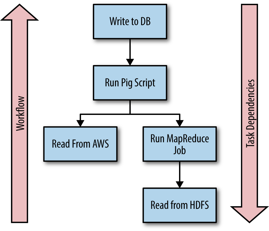
Tasks are the sequences of actions that comprise a Luigi workflow. Each task declares its dependencies on targets created by other tasks. This enables Luigi to create dependency chains that ensure a task will not be executed until all of the dependent tasks and all of the dependencies for those tasks are satisfied.
Figure 5-1 depicts a workflow highlighting Luigi tasks and their dependencies.
Target
Targets are the inputs and outputs of a task. The most common targets are files on a disk, files in HDFS, or records in a database. Luigi wraps the underlying filesystem operations to ensure that interactions with targets are atomic. This allows a workflow to be replayed from the point of failure without having to replay any of the already successfully completed tasks.
Parameters
Parameters allow the customization of tasks by enabling values to be passed into a task from the command line, programmatically, or from another task. For example, the name of a task’s output may be determined by a date passed into the task through a parameter.
An Example Workflow
This section describes a workflow that implements the WordCount algorithm to explain the interaction among tasks, targets, and parameters. The complete workflow is shown in Example 5-1.
Example 5-1. /python/Luigi/wordcount.py
import luigi

class InputFile(luigi.Task):
   """
   A task wrapping a target
   """
   input_file = luigi.Parameter()

   def output(self):
      """
      Return the target for this task
      """
      return luigi.LocalTarget(self.input_file)

class WordCount(luigi.Task):
   """
   A task that counts the number of words in a file
   """
   input_file = luigi.Parameter()
   output_file = luigi.Parameter(default='/tmp/wordcount')

   def requires(self):
      """
      The task's dependencies:
      """
      return InputFile(self.input_file)

   def output(self):
      """
      The task's output
      """
      return luigi.LocalTarget(self.output_file)

   def run(self):
      """
      The task's logic
      """
      count = {}

      ifp = self.input().open('r')

      for line in ifp:
         for word in line.strip().split():
            count[word] = count.get(word, 0) + 1

      ofp = self.output().open('w')
      for k, v in count.items():
            ofp.write('{}\t{}\n'.format(k, v))
      ofp.close()

if __name__ == '__main__':
   luigi.run()
This workflow contains two tasks: InputFile and WordCount. The InputFile task returns the input file to the WordCount task. The WordCount tasks then counts the occurrences of each word in the input file and stores the results in the output file.
Within each task, the requires(), output(), and run() methods can be overridden to customize a task’s behavior.
Task.requires
The requires() method is used to specify a task’s dependencies. The WordCount task requires the output of the InputFile task:
 def requires(self):
    return InputFile(self.input_file)
It is important to note that the requires() method cannot return a Target object. In this example, the Target object is wrapped in the InputFile task. Calling the InputFile task with the self.input_file argument enables the input_file parameter to be passed to the InputFile task.
Task.output
The output() method returns one or more Target objects. The InputFile task returns the Target object that was the input for the WordCount task:
def output(self):
   return luigi.LocalTarget(self.input_file)
The WordCount task returns the Target object that was the output for the workflow:
def output(self):
   return luigi.LocalTarget(self.output_file)
Task.run
The run() method contains the code for a task. After the requires() method completes, the run() method is executed. The run() method for the WordCount task reads data from the input file, counts the number of occurrences, and writes the results to an output file:
def run(self):
   count = {}

   ifp = self.input().open('r')

   for line in ifp:
      for word in line.strip().split():
         count[word] = count.get(word, 0) + 1

   ofp = self.output().open('w')
   for k, v in count.items():
      ofp.write('{}\t{}\n'.format(k, v))
   ofp.close()
The input() and output() methods are helper methods that allow the task to read and write to Target objects in the requires() and output() methods, respectively.
Parameters
Parameters enable values to be passed into a task, customizing the task’s execution. The WordCount task contains two parameters: input_file and output_file:
class WordCount(luigi.Task):
   input_file = luigi.Parameter()
   output_file = luigi.Parameter(default='/tmp/wordcount')
Default values can be set for parameters by using the default argument.
Luigi creates a command-line parser for each Parameter object, enabling values to be passed into the Luigi script on the command line, e.g., --input-file input.txt and --output-file /tmp/output.txt.
Execution
To enable execution from the command line, the following lines must be present in the application:
if __name__ == '__main__':
   luigi.run()
This will enable Luigi to read commands from the command line.
The following command will execute the workflow, reading from input.txt and storing the results in /tmp/wordcount.txt:
$ python wordcount.py WordCount \
--local-scheduler \
--input-file input.txt \
--output-file /tmp/wordcount.txt
Hadoop Workflows
This section contains workflows that control MapReduce and Pig jobs on a Hadoop cluster.
Configuration File
The examples in this section require a Luigi configuration file, client.cfg, to specify the location of the Hadoop streaming jar and the path to the Pig home directory. The config files should be in the current working directory, and an example of a config file is shown in Example 5-2.
Example 5-2. python/Luigi/client.cfg
[hadoop]
streaming-jar: /usr/lib/hadoop-xyz/hadoop-streaming-xyz-123.jar

[pig]
home: /usr/lib/pig
MapReduce in Luigi
Luigi scripts can control the execution of MapReduce jobs on a Hadoop cluster by using Hadoop streaming (Example 5-3).
Example 5-3. python/Luigi/luigi_mapreduce.py
import luigi
import luigi.contrib.hadoop
import luigi.contrib.hdfs

class InputFile(luigi.ExternalTask):
   """
   A task wrapping the HDFS target
   """
   input_file = luigi.Parameter()

   def output(self):
      """
      Return the target on HDFS
      """
      return luigi.contrib.hdfs.HdfsTarget(self.input_file)

class WordCount(luigi.contrib.hadoop.JobTask):
   """
   A task that uses Hadoop streaming to perform WordCount
   """
   input_file = luigi.Parameter()
   output_file = luigi.Parameter()

   # Set the number of reduce tasks
   n_reduce_tasks = 1

   def requires(self):
      """
      Read from the output of the InputFile task
      """
      return InputFile(self.input_file)

   def output(self):
      """
      Write the output to HDFS
      """
      return luigi.contrib.hdfs.HdfsTarget(self.output_file)

   def mapper(self, line):
      """
      Read each line and produce a word and 1
      """
      for word in line.strip().split():
         yield word, 1

   def reducer(self, key, values):
      """
      Read each word and produce the word and the sum of
      its values
      """
      yield key, sum(values)

if __name__ == '__main__':
   luigi.run(main_task_cls=WordCount)
Luigi comes packaged with support for Hadoop streaming. The task implementing the MapReduce job must subclass luigi.contrib.hadoop.JobTask. The mapper() and reducer() methods can be overridden to implement the map and reduce methods of a MapReduce job.
The following command will execute the workflow, reading from /user/hduser/input.txt and storing the results in /user/hduser/wordcount on HDFS:
$ python luigi_mapreduce.py --local-scheduler \
--input-file /user/hduser/input/input.txt \
--output-file /user/hduser/wordcount
Pig in Luigi
Luigi can be used to control the execution of Pig on a Hadoop cluster (Example 5-4).
Example 5-4. python/Luigi/luigi_pig.py
import luigi
import luigi.contrib.pig
import luigi.contrib.hdfs

class InputFile(luigi.ExternalTask):
   """
   A task wrapping the HDFS target
   """
   input_file = luigi.Parameter()

   def output(self):
      return luigi.contrib.hdfs.HdfsTarget(self.input_file)

class WordCount(luigi.contrib.pig.PigJobTask):
   """
   A task that uses Pig to perform WordCount
   """
   input_file = luigi.Parameter()
   output_file = luigi.Parameter()
   script_path = luigi.Parameter(default='pig/wordcount.pig')

   def requires(self):
      """
      Read from the output of the InputFile task
      """
      return InputFile(self.input_file)

   def output(self):
      """
      Write the output to HDFS
      """
      return luigi.contrib.hdfs.HdfsTarget(self.output_file)

   def pig_parameters(self):
      """
      A dictionary of parameters to pass to pig
      """
      return {'INPUT': self.input_file, 'OUTPUT': self.output_file}

   def pig_options(self):
      """
      A list of options to pass to pig
      """
      return ['-x', 'mapreduce']

   def pig_script_path(self):
      """
      The path to the pig script to run
      """
      return self.script_path

if __name__ == '__main__':
   luigi.run(main_task_cls=WordCount)
Luigi comes packaged with support for Pig. The task implementing the Pig job must subclass luigi.contrib.hadoop.PigJobTask. The pig_script_path() method is used to define the path to the Pig script to run. The pig_options() method is used to define the options to pass to the Pig script. The pig_parameters() method is used to pass parameters to the Pig script.
The following command will execute the workflow, reading from /user/hduser/input.txt and storing the results in /user/hduser/output on HDFS. The --script-path parameter is used to define the Pig script to execute:
$ python luigi_pig.py --local-scheduler \
--input-file /user/hduser/input/input.txt \
--output-file /user/hduser/output \
--script-path pig/wordcount.pig
Chapter Summary
This chapter introduced Luigi as a Python workflow scheduler. It described the components of a Luigi workflow and contained examples of using Luigi to control MapReduce jobs and Pig scripts.