 Lake Padarn Sunrise (source: Hefin Owen via Flickr)
 Leveraging Big Data Technologies to Build a Common Data Repository for Security
The term data lake comes from the big data community and is appearing in the security field more often. A data lake (or a data hub) is a central location where all security data is collected and stored; using a data lake is similar to log management or security information and event management (SIEM). In line with the Apache Hadoop big data movement, one of the objectives of a data lake is to run on commodity hardware and storage that is cheaper than special-purpose storage arrays or SANs. Furthermore, the lake should be accessible by third-party tools, processes, workflows, and to teams across the organization that need the data. In contrast, log management tools do not make it easy to access data through standard interfaces (APIs). They also do not provide a way to run arbitrary analytics code against the data.
Comparing Data Lakes to SIEM
Are data lakes and SIEM the same thing? In short, no. A data lake is not a replacement for SIEM. The concept of a data lake includes data storage and maybe some data processing; the purpose and function of a SIEM covers so much more.
The SIEM space was born out of the need to consolidate security data. SIEM architectures quickly showed their weakness by being incapable of scaling to the loads of IT data available, and log management stepped in to deal with the data volumes. Then the big data movement came about and started offering low-cost, open source alternatives to using log management tools. Technologies like Apache Lucene and Elasticsearch provide great log management alternatives that come with low or no licensing cost at all. The concept of the data lake is the next logical step in this evolution.
Implementing a Data Lake
Security data is often found stored in multiple copies across a company, and every security product collects and stores its own copy of the data. For example, tools working with network traffic (for example, IDS/IPS, DLP, and forensic tools) monitor, process, and store their own copies of the traffic. Behavioral monitoring, network anomaly detection, user scoring, correlation engines, and so forth all need a copy of the data to function. Every security solution is more or less collecting and storing the same data over and over again, resulting in multiple data copies.
The data lake tries to get rid of this duplication by collecting the data once, and making it available to all the tools and products that need it. This is much simpler said than done. The goal of this report is to discuss the issues surrounding and the approaches to architecting and implementing a data lake.
Overall, a data lake has four goals:
Provide one way (a process) to collect all data
Process, clean, and enrich the data in one location
Store data only once
Access the data using a standard interface
One of the main challenges of implementing a data lake is figuring out how to make all of the security products leverage the lake, instead of collecting and processing their own data. Products generally have to be rebuilt by the vendors to do so. Although this adoption might end up taking some time, we can work around this challenge already today.
Understanding Types of Data
When talking about data lakes, we have to talk about data. We can broadly distinguish two types of security data: time-series data, which is often transaction-centric, and contextual data, which is entity-centric.
Time-Series Data
The majority of security data falls into the category of time-series data, or log data. These logs are mostly single-line records containing a timestamp. Common examples come from firewalls, intrusion-detection systems, antivirus software, operating systems, proxies, and web servers. In some contexts, these logs are also called events, or alerts. Sometimes metrics or even transactions are communicated in log data.
Some data comes in binary form, which is harder to manage than textual logs. Packet captures (PCAPs) are one such source. This data source has slightly different requirements in the context of a data lake. Specifically because of its volume and complexity, we need clever ways of dealing with PCAPs (for further discussion of PCAPs, see the description on page 15).
Contextual Data
Contextual data (also referred to as context) provides information about specific objects of a log record. Objects can be machines, users, or applications. Each object has many attributes that can describe it. Machines, for example, can be characterized by IP addresses, host names, autonomous systems, geographic locations, or owners.
Let’s take NetFlow records as an example. These records contain IP addresses to describe the machines involved in the communication. We wouldn’t know anything more about the machines from the flows themselves. However, we can use an asset context to learn about the role of the machines. With that extra information, we can make more meaningful statements about the flows—for example, which ports our mail servers are using.
Contextual data can be contained in various places, including asset databases, configuration management systems, directories, or special-purpose applications (such as HR systems). Windows Active Directory is an example of a directory that holds information about users and machines. Asset databases can be used to find out information about machines, including their locations, owners, hardware specifications, and more.
Contextual data can also be derived from log records; DHCP is a good example. A log record is generated when a machine (represented by a MAC address) is assigned an IP address. By looking through the DHCP logs, we can build a lookup table for machines and their IP addresses at any point in time. If we also have access to some kind of authentication information—VPN logs, for example—we can then argue on a user level, instead of on an IP level. In the end, users attack systems, not IPs.
Other types of contextual data include vulnerability scans. They can be cumbersome to deal with, as they are often larger, structured documents (often in XML) that contain a lot of information about numerous machines. The information has to be carefully extracted from these documents and put into the object model describing the various assets and applications. In the same category as vulnerability scans, WHOIS data is another type of contextual data that can be hard to parse.
Contextual data in the form of threat intelligence is becoming more common. Threat feeds can contain information around various malicious or suspicious objects: IP addresses, files (in the form of MD5 checksums), and URLs. In the case of IP addresses, we need a mechanism to expire older entries. Some attributes of an entity apply for the lifetime of the entity, while others are transient. For example, a machine often stays malicious for only a certain period of time.
Contextual data is handled separately from log records because it requires a different storage model. Mostly the data is stored in a key-value store to allow for quick lookups. For further discussion of quick lookups, see page 17.
Choosing Where to Store Data
In the early days of the security monitoring, log management and SIEM products acted (and are still acting) as the data store for security data. Because of the technologies used 15 years ago when SIEMs were first developed, scalability has become an issue. It turns out that relational databases are not well suited for such large amounts of semistructured data. One reason is that relational databases can be optimized for either fast writes or fast reads, but not both (because of the use of indexes and the overhead introduced by the properties of transaction safety—ACID). In addition, the real-time correlation (rules) engines of SIEMs are bound to a single machine. With SIEMs, there is no way to distribute them across multiple machines. Therefore, data-ingestion rates are limited to a single machine, explaining why many SIEMs require really expensive and powerful hardware to run on. Obviously, we can implement tricks to mitigate the one-machine problem. In database land, the concept is called sharding, which splits the data stream into multiple streams that are then directed to separate machines. That way, the load is distributed. The problem with this approach is that the machines share no common “knowledge,” or no common state; they do not know what the other machines have seen. Assume, for example, that we are looking for failed logins and want to alert if more than five failed logins occur from the same source. If some log records are routed to different machines, each machine will see only a subset of the failed logins and each will wait until it has received five before triggering an alert.
In addition to the problem of scalability, openness is an issue of SIEMs. They were not built to let other products reuse the data they collected. Many SIEM users have implemented cumbersome ways to get the data out of SIEMs for further use. These functions typically must be performed manually and work for only a small set of data, not a bulk or continuous export of data.
Big-data technology has been attempting to provide solutions to the two main problems of SIEMs: scalability and openness. Often Hadoop is mentioned as that solution. Unfortunately, everybody talks about it, but not many people really know what is behind Hadoop.
To make the data lake more useful, we should consider the following questions:
Are we storing raw and/or processed records?
If we store processed records, what data format are we going to use?
Do we need to index the data to make data access quicker?
Are we storing context, and if so, how?
Are we enriching some of the records?
How will the data be accessed later?
Note
The question of raw versus processed data, as well as the specific data format, is one that can be answered only when considering how the data is accessed.
Knowing How Data Is Used
We need to consider five questions when choosing the right architecture for the back-end data store (note that they are all interrelated):
How much data do we have in total?
How fast does the data need to be ready?
How much data do we query at a time, and how often do we query?
Where is the data located, and where does it come from?
What do you want to do with the data, and how do you access it?
How Much Data Do We Have in Total?
Just because everyone is talking about Hadoop doesn’t necessarily mean we need a big data solution to store our data. We can store multiple terabytes in a relational database, such as MySQL. Even if we need multiple machines to deal with the data and load, often sharding can help.
How Fast Does the Data Need to Be Ready?
In some cases, we need results immediately. If we drive an interactive application, data-retrieval rates often need to be completed at subsecond speed. In other cases, it is OK to have the result available the next day. Determining how fast the data needs to be ready can make a huge difference in how it needs to be stored.
How Much Data Do We Query, and How Often?
If we need to run all of our queries over all of our data, that is a completely different use-case from querying a small set of data every now and then. In the former case, we will likely need some kind of caching and/or aggregate layer that stores precomputed data so that we don’t have to query all the data at all times. An example is a query for a summary of the number of records seen per user per hour. We would compute those aggregates every hour and store them. Later, when we want to know the number of records that each user looked at last week, we can just query the aggregates, which will be much faster.
Where Is the Data and Where Does It Come From?
Data originates from many places. Some data sources write logs to files, others can forward data to a network destination (for example, through syslog), and some store records in a database. In some cases, we do not want to move the data if it is already stored in some kind of database and it supports our access use-case; this concept is sometimes called a federated data store.
What Do You Want with the Data and How Do You Access It?
While we won’t be able to enumerate every single use case for querying data, we can organize the access paradigms into five groups:
- Search
- Data is accessed through full-text search. The user looks for arbitrary text in the data. Often Boolean operators are used to structure more advanced searches.
- Analytics
These queries require slicing and dicing the data in various ways, such as summing columns (for example, for sales prices). There are three subgroups:
- Record-based analytics
- These use cases entail all of the traditional questions we would ask a relational database. Business intelligence questions, for example, are great use cases for this type of analytics.
- Relationships
- These queries deal with complex objects and their relationships. Instead of looking at the data on a record-by-record (or row) basis, we take an object-centric view, where objects are anything from machines to users to applications. For example, when looking at machine communications, we might want to ask what machines have been communicating with machines that our desktop computer has accessed. How many bytes were transferred, and how long did each communication last? These are queries that require joining log records to come up with the answers to these types of questions.
- Data mining
- This type of query is about running jobs (algorithms) against a large set of our data. Unlike in the case of simple statistics, where we might count or do simple math, analytics or data-mining algorithms that cluster, score, or classify data fall into this category. We don’t want to pull all the data back to one node for processing/analytics; instead, we want to push the code down to the individual nodes to compute results. Many hard problems are related to data locality, and communication between nodes to exchange state, for example, that need to be considered for this use case (but essentially, this is what a distributed processing framework is for).
- Raw data access
- Often we need to be able to go back to the raw data records to answer more questions with data that is part of the raw record but was not captured in parsed data.
- These access use cases are focused around data at rest—data we have already collected. The next two are use cases in the real-time scenario.
- Real-time statistics
- The raw data is not always what we need or want. Driving dashboards, for example, require metrics or statistics. In the simplest cases of real-time scenarios, we count things—for example, the number of events we have ingested, the number of bytes that have been transferred, or the number of machines that have been seen. Instead of calculating those metrics every time a dashboard is loaded—which would require scanning a lot of the data repeatedly—we can calculate those metrics at the time of collection and store them so they are readily available. Some people have suggested calling this a data river.
- A commonly found use case in computer security is scoring of entities. Running models to identify how suspicious or malicious a user is, for example, can be done in real time at data ingestion.
- Real-time correlation
- Real-time correlation, rules, and alerting are all synonymous. Correlation engines are often referred to as complex event processing (CEP) engines; there are many ways of implementing them. One use case for CEP engines is to find a known pattern based on the definition of hard-coded rules; these systems need a notion of state to remember what they have already seen. Trying to run these engines in distributed environments gets interesting, especially when you consider how state is shared among nodes.
Storing Data
Now that you understand the options for where to store the data and the access use-cases, we can now dive a little deeper into which technologies you might use to store the data and how exactly it is stored.
Using Parsers
Before we dive into details of how to store data, we need to discuss parsers. Most analysis requires parsed, or structured, data. We therefore need a way to transform our raw records into structured data. Fields (such as port numbers or IP addresses) inside a log record are often self-evident. At times, it’s important to figure out which field is the source address and which one is the destination. In some cases, however, identifying fields in a log record is impossible without additional knowledge. For example, let’s assume that a log record contains a number, with no key to identify it. This number could be anything: the number of packets transmitted, number of bytes transmitted, or number of failed attempts. We need additional knowledge to make sense of this number. This is where a parser adds value. This is also why it is hard and resource-intensive to write parsers. We have to gather documentation for the data source to learn about the format and correctly identify the fields. Most often, parsers are defined as regular expressions, which, if poorly written or under heavy load, can place a significant burden on the parsing system.
All kinds of off-the-shelf products claim that they don’t need parsers. But the example just outlined shows that at some point, a parser is needed (unless the data already comes in some kind of a structured form).
We need to keep two more things in mind. First, parsing doesn’t mean that the entire log record has to be parsed. Depending on the use case, it is enough to parse only some of the fields, such as the usernames, IP addresses, or ports. Second, when parsing data from different data sources, a common field dictionary needs to be used; this is also referred to as an ontology (which is a little more than just a field dictionary). All the field dictionary does is standardize the names across data sources. An IP address can be known by many names, such as: sourceAddress, sourceIP, srcIP, and src_ip. Imagine, for example, a setup where parsers use all of these names in the same system. How would you write a query that looked for addresses across all these fields? You would end up writing this crazy chain of ORed-together terms; that’s just ugly.
One last thing about parsing: we have three approaches to parsing data:
- Collection-time parsing
- In collection-time parsing, the data is parsed as soon as it is collected. All processing is then done on parsed, or structured, data—enabling all kinds of analytical use-cases. The disadvantage is that parsers have to be available up front, and if there is a mistake or an omission in the parsers, that data won’t be available.
- Batch parsing
- In batch parsing, the data is first stored in raw form. A batch process is then used to parse the data at regular intervals. This could be done once a day or once a minute, depending on the requirements. Batch parsing is similar to collection-time parsing in that it requires parsers up front, and after the data is parsed, it is often hard to change. However, batch parsing has the potential to allow for reparsing and updating the already-parsed records. We need to watch out for a few things, though—for example, computations that were made over “older” versions of the parsed data. Say we didn’t parse the username field before. All of our statistics related to users wouldn’t take these records into account. But now that we are parsing this field, those statistics should be taken into account as well. If we haven’t planned for a way to update the old stats in our application, those numbers will now be inconsistent.
- Process-time parsing
- Process-time parsing collects data in its raw form. If analytical questions are involved, the data is then parsed at processing time. This can be quite inefficient if large amounts of data are queried. The advantage of this approach is that the parsers can be changed at any point in time. They can be updated and augmented, making parsing really flexible. It also is not necessary to know the parsers up front. The biggest disadvantage here is that it is not possible to do any ingest-time statistics or analytics.
Overall, keep in mind that the topic of parsing has many more facets we don’t discuss here. Normalization may be needed if numerous data sources call the same action by different names (for example, “block,” “deny,” and “denied” are all names found in firewall logs for communications that are blocked). Another related topic is value normalization, used to normalize different scales. (For example, one data source might use a high, medium, or low rating, while another uses a scale from 1 to 10.)
Storing Log Data
To discuss how to store data, let’s revisit the access use cases we covered earlier (see What Do You Want with the Data and How Do You Access It?), and for each of them, discuss how to approach data storage.
Search
Getting fast access based on search queries requires an index. There are two ways to index data: full-text or token-based. Full text is self-explanatory; the engine finds tokens in the data automatically, and any token or word it finds it will add to the index. For example, think of parsing a sentence into words and indexing every word. The issue with this approach is that the individual parts of the sentence or log record are not named; all the words are treated the same. We can leverage parsers to name each token in the logs. That way, we can ask the index questions like username = rmarty, which is more specific than searching all records for rmarty.
The topic of search is much bigger with concepts like prefix parsing and analyzers, but we will leave it at this for now.
Analytics
Each of the three subcases in analytics require parsed, or structured, data. Following are some of the issues that need to be taken into consideration when designing a data store for analytics use-cases:
What is the schema for the data?
Do we distribute the data across different stores/tables? Do some workloads require joining data from different tables? To speed up access, does it make sense to denormalize the database tables?
Does the schema change over time? How does it change? Are there only additions or also deletions of columns/fields? How many? How often does that occur?
Speed is an important topic that has many facets. Even with a well thought-out schema and all kinds of optimizations, queries can still take a long time to return data. A caching layer can be introduced to store the most accessed data or the most returned results. Sometimes database engines have a caching layer built in; sometimes an extra layer is added. A significant factor is obviously the size of the machines in use; the more memory, the faster the processors (or the more processors), and the faster the network between nodes, the quicker the results will come back (in general).
If a single node cannot store all of the data, the way that the data is split across multiple nodes becomes relevant. Partitioning the data, when done right, can significantly increase query speeds (because the query can be restricted to only the relevant partitions) and data management (allowing for archiving data).
Following is a closer look at the three sub-uses of analytics:
- Record-based analytics
- Parsed data is stored in a schema-based/structured data store, where you can choose either a row-based or columnar storage format. Most often, columnar storage is more efficient and faster for relational queries, such as counts, distinct counts, sums, and group-bys. Columnar storage also has better compression rates than row-based stores. We should bear in mind a couple of additional questions when designing a relational store:
Are we willing to sacrifice some speed in return for the flexibility of schemas on demand? Big-data stores like Hive and Impala let the user define schemas at query time; in conjunction with external tables, this makes for a fairly flexible solution. However, the drawback is that we embed the parsers in every single query, which does not really scale.
Some queries can be sped up by computing aggregates; online analytical processing (OLAP) cubes fall into this area. Instead of computing certain statistical results over and over, OLAP cubes are computed and stored before the result is needed.
- Relationships
- Log records are broken into the objects and relationships between them, or in graph terms, with nodes and edges connecting them. Nodes are entities such as machines, users, applications, files, and websites; these entities are linked through edges. For example, an edge would connect the nodes representing applications and the machines these applications are installed on. Graphs let the user express more complicated, graph-related queries—such as “show me all executables executed on a Windows machine that were downloaded in an email.” In a relational store, this type of query would be quite inefficient. First, we would have to go through all emails and see which ones had attachments. Then we’d look for executables. With this candidate set, we’d then query the operating system logs to find executables that have been executed on a Windows machine. By using graphs, much longer chains of reasoning can be constructed that would be really hard to express in a relational model. Beware that most analytical queries will be much slower in a graph, though, than in a relational store.
- Distributed processing
- We sometimes need to run analytics code on all or a significant subset of our data. An example of such jobs are clustering approaches that find groups of similar items in the data. The naive approach would be to find the relevant data and bring it back to one node where the analytics code is run; this can be a large amount of data if the query is not very discriminating. The more efficient approach is to bring the computation to the data; this is the core premise of the MapReduce paradigm.
- Common applications for distributed processing are clustering, dimensionality reduction, and classifications—data-mining approaches in general.
Raw Data
When processing/parsing data, we end up storing the parsed data in some kind of a structured store. The question remains of what to do with the raw data. The following are a few reasons we would want to keep the raw data:
In case we need to reparse the data, especially if the parsing was incomplete or the parsers were wrong.
The raw data needs to be shown to the user.
Other data-processing steps will need raw data—for example, natural language processing (NLP) or sentiment analysis.
Raw data is required to be stored by compliance or regulatory mandates.
Packet captures (PCAP) are a special case of raw data. They are large because they contain all of the network conversations. There are a few recommendations when it comes to storing PCAPs:
Parse out as much meta information from the raw packets as possible and necessary: extract IP addresses, ports, URLs, and so forth and store them in a structured store for query and analytics. When doing so, make sure to point the metadata back to the full-packet captures; that way, you can search the metadata and find the corresponding packets for further details. You can also keep the meta information around longer than the large PCAPs; most analytics will run on the metadata anyway.
Store/capture PCAPs for a short amount of time; short is relative and can mean anything from a couple of hours to a couple of weeks. This data can be used for in-depth forensics investigations if the metadata collected and extracted is not enough.
For specific areas of the network—for example, communications involving critical servers—store the raw packets for a longer period of time.
One thing to keep in mind is that all of the preceding cases are not mutually exclusive. In fact, most of the time, we will need all of the access use cases. Therefore, we will end up needing a data store that supports all of these approaches. We will discuss technologies and specific data stores in Accessing Data; first we have to address one more topic: storing context.
Storing Context
We mentioned earlier that context, or contextual data, is slightly special. One option is to store context in a graph database by attaching the context as properties of individual objects. What if we want or need to use one of the other data stores? How do we leverage context for search, analytics, and data mining (distributed processing)? For example, we might want to search for all of the records that involve web servers. The data records themselves contain only IP addresses and no machine roles. The context, however, consists of a mapping from IP addresses to machine roles. Or we might want to compute some kind of statistics for web servers.
We can take two approaches to incorporate context for those cases:
- Enrich at collection time
- The first option is to augment every record at ingestion time. When the data is collected, we add the extra information to each record. This puts more load on the input processing and definitely consumes more storage on the back end, because every record now contains extra columns with the context. The benefit is that we can easily run any analytics/search right against the main data without any lookups. The caveat is that enrichment at collection time works only for context that does not change over time.
- Enrich in batch: Instead of doing all of the enrichment in real time when data is collected, we can also run batch jobs over all of the data to enrich it anytime after it’s collected.
- Join at processing time
- The other option, if the overhead of enrichment is too high, is to join the data at processing time. Let’s take our example from earlier. We would first use the context store to find all the IP addresses of web servers. We would then take that list to query against the main data store to find all the records that involve those IP addresses. Depending on the size of the list of IP addresses (how many web servers there are), this can get pretty expensive in terms of processing time. In a relational data store that supports joins, we can normalize the schema and store the context in a separate table that is then joined against the main data table whenever needed.
Either or both of the preceding approaches can be right, depending on the situation. Most likely, you will end up with a hybrid approach, whereby some of the data should be enriched at collection time, some on a regular basis in batch, and some that is looked up in real time. The decision depends on how often we use the information and how expensive the query becomes if we do a real-time lookup.
Ideally, we implement a three-tier system:
Real-time lookup table: Lookups are often stored in key-value stores, which are really fast at finding associations for a key. Keep in mind that the reverse—looking up a key for a given value—is not easily possible. However, a method called an inverse index, which some key-value stores support out of the box, will facilitate this task. In other cases, you will have to add the inverse index (value→key) manually. In a relational database, you can store the lookups in a separate table. In addition, you might want to index the columns for which you issue a lot of lookups. Also, keep in mind that some lookups are valid at only certain times, so keep a time range with the data that defines the validity of the lookup. For example, a DHCP lease is valid for only a specific time period and might change afterward.
In-memory cache: Some lookups we have to repeat over and over again, and hitting disks to answer these queries is inefficient. Figure out which lookups you do a lot and cache those values in memory. This cache can be an explicit caching layer (something like memcache), or could be part of whatever key-value store we use to store the lookups.
Enrich data: The third tier is to enrich the data itself. Most likely there will be some data fields for which we have to do this to get decent query times across analytical and search operations. Ideally, we’d be able to instrument our applications to see what kinds of fields we need a lot and then enrich the data store with that information—an auto-adopting system.
Accessing Data
How is data accessed after it is stored? Every data store has its own ways of making the data available. SQL used to be the standard for interacting with data, until the NoSQL movement showed up. APIs were introduced that didn’t need SQL but instead used a proprietary language to query data. It is interesting to observe, however, that many of those NoSQL stores have introduced languages that look very much like SQL, and, in a lot of cases, now support SQL-compliant interfaces. It is a good policy to try to find data stores that support SQL as a query language. SQL is expressive (it allows for many data-processing questions) and is known by a lot of programmers and even business analysts (and security analysts, for that matter). Many third-party tools and products also allow interfacing with SQL-based data stores, which makes integrations easier.
Another standard that is mentioned often, along with SQL, is JDBC. JDBC is a commonly used transport protocol to access SQL-based data stores. Libraries are available for many programming languages, and many products embed a JDBC driver to hook into the database. Both SQL and JDBC are standards that you should have an eye out for.
RESTful APIs are not a good option to access data. REST does not define a query language for data access. If we defined an interface, we would have to make sure that the third-party tools would understand them. If the data lake was used by only our own applications, we could go this route, but bearing in mind that this would not scale to third-party products.
Figure 1-1 shows a flow diagram with the components we discussed in this section.
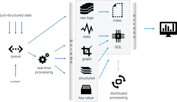
The components are as follows:
The real-time processing piece contains parts of parsing, as well as the aggregation logic to feed the structured stores. It would also contain any behavioral monitoring, or scoring of entities, as well as the rule-based real-time correlation engine.
The data lake itself spans the gray box in the middle of Figure 1-1. The distributed processing piece could live in your data lake, as well as other components not shown here.
The access layer often consists of some kind of a SQL interface. However, it doesn’t have to be SQL; it could be anything else, like a RESTful interface, for example. Keep in mind, though, that using non-SQL will make integrating with third-party products more difficult; they would have to be built around those interfaces, which is most likely not an option.
The storage layer could be HDFS to share data across all the components (key-value store, structured store, graph store, stats store, raw data storage), but often you will end up with multiple, separate data stores for each of the components. For example, we might have a columnar store for the structured data already—something like Vertica, TeraData, or Hexis. These stores will most likely not have the data stored on HDFS in a way that other data stores could access them, and you will need to create a separate copy of the data for the other components.
The distributed processing component contains any logic that is used for batch processing. In the broadest sense, we can also lump batch processes (for example, later-stage enrichments or parsing) into this component.
Based on the particular access use case, some of the boxes (data stores) won’t be needed. For example, if search is not a use case, we won’t need the index, and likely won’t need the graph store or the raw logs.
Ingesting Data
Getting the data into the data lake consists of a few parts:
- Parsing
- We discussed parsing at length already (see Using Parsers). Keep a few things in mind: SIEMs have spent a lot of time building connectors/agents (or collectors), which are basically parsers. Both the transport to access the data (such as syslog, WMF) and the data structure (the syntax of the log messages) take a lot of time to be built across the data sources. Don’t underestimate the work involved in this. If there is a way to reuse the parsers of a SIEM, you should!
- Enrichment
- We discussed enrichment at length earlier (see page 16). As an example, DNS resolution is often done at ingestion time to resolve IP addresses to host names, and the other way around. This makes it possible to correlate data sources that have either of those data fields, but not both. Consider, however, that a DNS lookup can be really slow. Holding up the ingestion pipeline to wait for a DNS response might not always be possible. Most likely, you should have a separate DNS server to answer these lookups, or consider the enrichment after the fact based on a batch job.
- In the broadest sense, matching the real-time log feed against a list of indicators of compromise (IOC) can be considered enrichment as well.
- Federated data
- We talked a little about federated data stores (see Where Is the Data and Where Does It Come From?). If you have an access layer that allows for data to be distributed in different stores, that might be a viable option, instead of reading the data from the original stores and forwarding it into the data lake.
- Aggregation
- As we are ingesting data into the data lake, we can already begin some real-time statistics, by computing various types of statistical summaries. For example, counting events and aggregating data by source address are two types of summaries we can create during ingestion, which can speed up queries for those summaries later.
- Third-party access
- Third-party products might need access to your real-time feed in order to do their own processing. Jobs like scoring and behavioral models, for example, often require access to a real-time feed. You will either need a way to forward a feed to those tools, or run those models through your own infrastructure, which opens up a number of new questions about how exactly to enable the feed.
Understanding How SIEM Fits In
SIEMs get in trouble for three main issues: actual threat detection, scalability, and storage of advanced context, such as HR data. The one main issue we can try to address with the data lake is scalability. We have seen expensive projects try to replace their SIEM with some big data/Hadoop infrastructure, just for the team to realize that some SIEM features would be really hard to replicate.
In order to decide which parts of an SIEM could be replaced with the aid of some additional plumbing, first we must look at SIEM’s key capabilities, which include the following:
Rich parsers for a large set of security data sources
Mature parsing and enrichment framework
Real-time, stateful correlation engine (generally not distributed)
Real-time statistical engine
Event triage and workflow engines
Dashboards and reports
User interfaces to configure real-time engines
Search interface for forensics
Ticketing and case management system
Given that this is a fairly elaborate list, instead of replacing the SIEM, it might make more sense to embed the SIEM into your data-lake strategy. There are a couple of ways to do so, each having its own caveats. Review Table 1-1 for a summary of the four main building blocks that can be used to put together a SIEM–data lake integration.
We will use the four main building blocks described in Table 1-1 to discuss four additional, more elaborate use cases based on these building blocks:
Traditional data lake
Preprocessed data
Split collection
Federated data access
 |
Traditional Data Lake
Whatever data possible is stored in its raw form on HDFS. From there, it is picked up and forwarded into the SIEM, applying some filters to reduce the amount of data collected via the SIEM (see Figure 1-2).
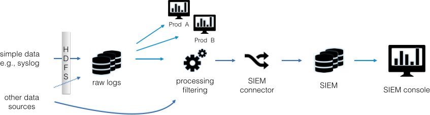
The one main benefit of this architecture is that we can significantly reduce the effort of getting access to data for security monitoring tools. Without such a central setup, each new security monitoring tool needs to be fed a copy of the original data, which results in getting other teams involved to make configuration changes to products, making changes to production infrastructure that are risky, and having some data sources that might not support copying their data to multiple destinations. In the traditional data lake setup, data access can be handled in one place. However, this architecture has a few disadvantages:
We need transport agents that can read the data at its origin and store it in HDFS. A tool called Apache Flume is a good option.
Each product that wants to access the data lake (the raw data) needs a way to read the data from HDFS.
Parsing has to be done by each product independently, thereby duplicating work across all of the products.
When picking up the data and forwarding it to the SIEM (or any other product), the SIEM needs to understand the data format (syntax). However, most SIEM connectors (and products) are built such that a specific connector (say for Check Point Firewall) assumes a specific transport to be present (OPSEC in our example) and then expects a certain data format. In this scenario, the transport would not be correct.
For other data sources that we cannot store in HDFS, we have to get the SIEM connectors to directly read the data from the source (or forward the data there). In Figure 1-2 we show an arrow with a dotted line, where it might be possible to send a copy of the data into the raw data store as well.
As you can see, the traditional data lake setup doesn’t have many benefits. Hardly any products can read from the data lake (that is, HDFS), and it is hard to get the SIEMs to read from it too. Therefore, a different architecture is often chosen, whereby data is preprocessed before being collected.
Preprocessed Data
The preprocessed data architecture collects data in a structured or semistructured data store, before it is forwarded to the SIEM. Often this precollection is done either in a log management, or some other kind, of data warehouse, such as a columnar database. The data store is used to either summarize the data and forward summarized information to the SIEM, or to forward a filtered data stream in order to not overload the SIEM (see Figure 1-3).
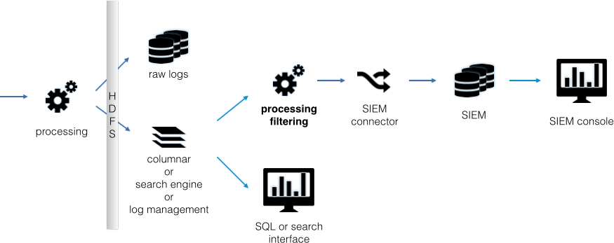
The reasons for using a preprocessed data setup include the following:
Reduces the load on the SIEM by forwarding only partial information, or forwarding presummarized information.
Collects the data in a standard data store that can be used for other purposes; often accessible via SQL.
Stores data in an HDFS cluster for use with other big data tools.
Leverages cheaper data storage to collect data for archiving purposes.
Frequently chosen if there is already a data warehouse, or a relational data store available for reuse.
As with a traditional data lake, some of the challenges with using the preprocessed data setup include the following:
You will need a way to parse the data before collection. Often this means that the SIEM’s connectors are not usable.
The SIEM needs to understand the data forwarded from the structured store. This can be a big issue, as discussed previously. If the SIEM supports a common log format, such as the Common Event Format (CEF), we can format the data in that format and send it to the SIEM.
Split Collection
The split collection architecture works only if the SIEM connector supports forwarding textual data to a text-based data receiver in parallel to sending the data to the SIEM. You would configure the SIEM connector to send the data to both the SIEM and to a process, such as Flume, logstash, or rsyslog, that can write data to HDFS, and then store the data in HDFS as flat files. Make sure to partition the data into directories to allow for easy data management. A directory per day and a file per hour is a good start until the files get too big, and then you might want to have directories per hour and a file per hour (see Figure 1-4).

Some of the challenges with using split collection include the following:
The SIEM connector needs to have two capabilities: forwarding textual information and copying data to multiple destinations.
If raw data is forwarded to HDFS, we need a place to parse the data. We can do this in a batch process (MapReduce job) over HDFS. Alternatively, some SIEM connectors are capable of forwarding data in a standardized way, such as in CEF format. (Having all of the data stored in a standard format in HDFS makes it easy to parse later.)
If you are running advanced analytics outside the SIEM, you will have to consider how the newly discovered insight gets integrated back into the SIEM workflow.
Federated Data Access
It would be great if we could store all of our data in the data lake, whether it be security-related data, network metrics (the SNMP input in the diagram), or even HR data. Unlike in our first scenario (the traditional data lake), the data collected is not in raw form anymore. Instead, we’re collecting processed data (see Figure 1-5).
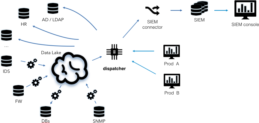
To enable access to the data, a “dispatcher” is needed to orchestrate the data access. As shown in Figure 1-5, not all data is forwarded to the lake. Some data is kept in its original store, and is accessed remotely by the dispatcher when needed.
Some of the challenges with using federated data access include the following:
There is no off-the-shelf dispatcher available; you will need to implement this capability yourself. It needs to support both batch data access (probably through SQL), but also a real-time streaming capability to forward data to any kind of real-time system, such as your SIEM.
Security products (such as behavior analytics tools, visualization tools, and search interfaces) need to be rewritten to leverage the dispatcher.
Accessing data in a federated way (for example, HR data) might not be possible or may be hard to implement (for example, schemas need to be understood or systems need to allow third-party access).
Controlling access to and protecting the data store becomes a central security problem, and any data-lake project will need to address these issues.
Despite all of the challenges with a federated data access setup, the benefits of such an architecture are quite interesting:
Data is collected only once.
Data from critical systems, such as an HR system, can be left in its original data store.
The data lake can be leveraged by not only the security teams, but also any other function in the company that needs access to the same data.
A fifth setup consists of first collecting the data in a SIEM and then extracting it to feed it into the security data lake. This setup is somewhat against the principle of the data lake, in that it first collects the data in a big data setup and then gives third-party tools (among them the SIEM) access. In addition, most SIEMs do not have a good way to get data out of their data store.
Acknowledgments
I would like to thank all of the people who have provided input to early ideas and versions of this report. Special thanks go to Jose Nazario, Anton Chuvakin, and Charaka Goonatilake for their great input that has made this report what it is.
Appendix: Technologies To Know and Use
The following list briefly summarizes a few key technologies (for further reading, check out the Field Guide to Hadoop):
- HDFS
- A distributed file system supporting fault tolerance and replication.
- Apache MapReduce
- A framework that allows for distributed computations. One of the core ideas is to bring processing to the data, instead of data to the processor. An algorithm has to be broken into map and reduce components that can be strung together in arbitrary topologies to compute results over large amounts of data. This can become quite complicated, and optimizations are left to the programmer. Newer frameworks exist that abstract the MapReduce subtasks from the programmer. The framework is used to optimize the processing pipeline. Spark is such a framework.
- YARN
- Yet Another Resource Negotiator (YARN), sometimes also called MapReduce 2.0, is a resource manager and job scheduler. It is an integral part of Hadoop 2, which basically decouples HDFS from MapReduce. This allows for running non-MapReduce jobs in the Hadoop framework, such as streaming and interactive querying.
- Spark
- Just like MapReduce, Spark is a distributed processing framework. It is part of the Berkeley Data Analytics Stack (BDAS), which encompasses a number of components for big data processing both in real time, as well as batch uses. Spark, which is the core component of the BDAS stack, supports arbitrary algorithms to be run in a distributed environment. It makes efficient use of memories on the compute nodes and will cache on disk if needed. For structured data processing needs, SparkSQL is used to interact with the data through a SQL interface. In addition, a Spark Streaming component allows for real-time processing (microbatching) of incoming data.
- Hive
- An implementation of a query engine for structure data on top of MapReduce. In practice, this means that the user can write HQL (for all intended purposes, it’s SQL) queries against data stored on HDFS. The drawback of Hive is the query speed because it invokes MapReduce as an underlying computation engine.
- Impala, Hawk, Stinger, Drill
- Interactive SQL interfaces for data stored in HDFS. They are trying to match the capabilities of Hive, but without using MapReduce as the computation engine—making SQL queries much faster. Each of the four has similar capabilities.
- Key-value stores
- Data storage engines that store data as key-value pairs. They allow for really fast lookup of values based on their keys. Most key-value stores add advanced capabilities, such as inverse indexes, query languages, and auto sharding. Examples of key-value stores are Cassandra, MongoDB, and HBase.
- Elasticsearch
A search engine based on the open source search engine Lucene. Documents are sent to Elasticsearch (ES) in JSON format. The engine then creates a full-text index of the data. All kinds of configurations can be tweaked to tune the indexing and storage of the indexed documents. While search engines call their unit of operation a document, log records can be considered documents. Another search engine is Solr, but ES seems to be used more in log management.
- ELK stack
- A combination of three open source projects: Elasticsearch, logstash, and Kibana. Logstash is responsible for collecting log files and storing them in Elasticsearch (it has a parsing engine), Elasticsearch is the data store, and Kibana is the web interface to build dashboards and query the data stored in Elasticsearch.
- Graph databases
- A database that models data as nodes and edges (for example, as a graph). Examples include Titan, GraphX, and Neo4j.
- Apache Storm
- A real-time, distributed processing engine just like Spark Streaming.
- Columnar data store
- We have to differentiate between the query engines themselves (such as Impala, Hawk, Stinger, Drill, and Hive) and how the data is stored. The query engines can use various kinds of storage engines. Among them are columnar storage engines such as parquet, and Optimized Row Columnar (ORC) files; these formats are self-describing, meaning that they encode the schema along with the data.
A good place to start with the preceding technologies is one of the big data distributions from Cloudera, Hortonworks, MapR, or Pivotal. These companies provide entire stacks of software components to enable a data lake setup. Each company also makes a virtual machine available that is ready to go and can be used to easily explore the components. The distributions differ mainly in terms of management interfaces, and strangely enough, in their interactive SQL data stores. Each vendor has its own version of an interactive SQL store, such as Impala, Stinger, Drill, and Hawk.
Finding qualified resources that can help build a data lake is one of the toughest tasks you will have while building your data stack. You will need people with knowledge of all of these technologies to build out a detailed architecture. Developer skills—generally, Scala or Java skills in the big data world—will be necessary to fill in the gaps between the building blocks. You will also need a team with system administration or devops skills to build the systems and to deploy, tune, and monitor them.