Time-series analysis on cloud infrastructure metrics

Many businesses are choosing to migrate, or natively build their infrastructure in the cloud; doing so helps them realize a myriad of benefits. Among these benefits is the ability to lower costs by “right-sizing” infrastructure, to adequately meet demand without under- or over-provisioning. For businesses with time-varying resource needs, the ability to “spin-up” and “spin-down” resources based on real-time demand can lead to significant cost savings.

Major cloud-hosting providers like Amazon Web Services (AWS) offer management tools to enable customers to scale their infrastructure to current demand. However, fully embracing such capabilities, such as AWS Auto Scaling, typically requires:

1. Optimized Auto Scaling configuration that can match customer’s application resource demands
2. Potential cost saving and business ROI

Attempting to understand potential savings from the use of dynamic infrastructure sizing is not a trivial task. AWS’s Auto Scaling capability offers a myriad of options, including resource scheduling and usage-based changes in infrastructure. Businesses must undertake detailed analyses of their applications to understand how best to utilize Auto Scaling, and further analysis to estimate cost savings.

In this article, we will discuss the approach we use at Datapipe to help customers customize Auto Scaling, including the analyses we’ve done, and to estimate potential savings. In addition to that, we aim to demonstrate the benefits of applying data science skills to the infrastructure operational metrics. We believe what we’re demonstrating here can also be applied to other operational metrics and hope our readers can apply the same approach to their own infrastructure data.

Infrastructure usage data

We approach Auto Scaling configuration optimization by considering a recent client project, where we helped our client realize potential cost savings by finding the most optimized configuration. When we initially engaged with the client, their existing web-application infrastructure consisted of a static and fixed number of AWS instances running at all times. However, after analyzing their historical resource usage patterns, we observed that the application had time-varying CPU usage, where at times, the AWS instances were barely utilized. In this article, we will analyze simulated data that closely matches the customer’s usage patterns, but preserves their privacy.

In Figure 1, we show two weeks’ worth of usage data, similar to that available from Amazon’s CloudWatch reporting/monitoring service, which allows you to collect infrastructure related metrics:

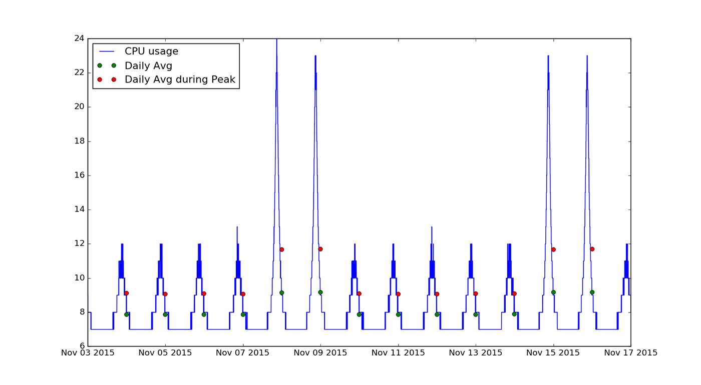
A quick visual inspection reveals two key findings:

• Demand for the application is significantly higher during late evenings and nights. During other parts of the day, it remains constant.
• There is a substantial increase in demand over the weekend.

A bit more analysis will allow us to better understand these findings. Let’s look at the weekend usage (Saturday–Sunday) and the weekday usage (Monday–Friday), independently. To get a better sense of the uniformity of the daily cycle within each of these two groups, we can aggregate the data to compare the pattern on each day. To do so, we binned the data into regular five-minute intervals throughout the 24 hour day (e.g., 0:00, 0:05, etc.) and determined the minimum, maximum, and average for each of these intervals.

Note that for this example, since the peak period extends slightly past midnight, we defined a “day” as spanning from noon-noon across calendar dates. The difference between the weekday group (red) and the weekend group (blue) is seen quite starkly in the plot below. The dotted lines show the minimum and maximum usage envelopes around the average, which is shown with the solid line:

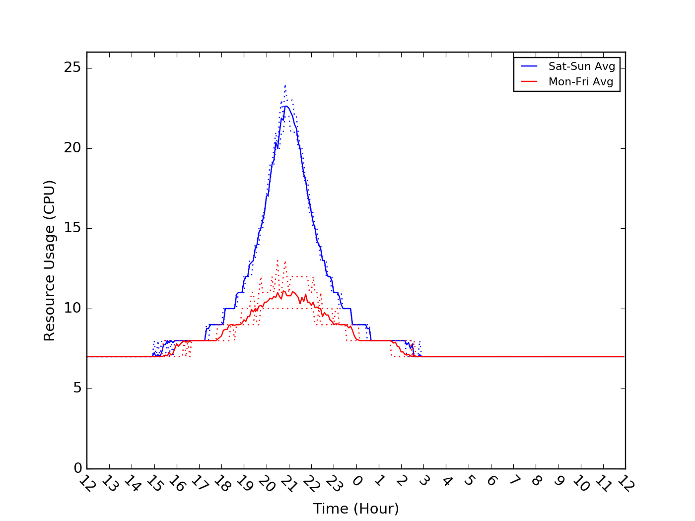
In this example, it is also visually apparent that the minimum and maximum envelopes hew very closely to the average usage cycles for both the weekend and weekday groups—indicating that, over this two week period, the daily cycles are very consistent. If the envelope were wider, we could examine additional metrics, such as standard deviation, 1st and 3rd quartiles, or other percentiles (e.g., 10th and 90th or 1st and 99th), to get a sense for how consistent the usage cycle is from day to day.

Although not evident in this example, another frequent consideration when examining infrastructure usage is assessing whether there is an overall increase or decrease in usage over time. For a web-based software application, such changes could indicate growth or contraction of its user base, or reveal issues with the software implementation, such as memory leaks. The lack of such trends in this data is apparent upon visual inspection, but there are some simple quantitative techniques we can use to verify this theory.

One approach is to find the average usage for each day in the data set and determine whether there is a trend for these values within either the weekday or the weekend groupings. These daily averages are plotted in green in Figure 1. In this example, it is obvious by eye that there is no trend; however, this can also be verified by fitting a line to the values in each set. We find that for both groupings, the slope is consistent with zero, indicating no change in the average daily usage over this two-week period. However, because of the cyclical nature of the usage pattern, we may be concerned that the long periods of low, constant usage might overwhelm any trends during the peak periods. To test this, we can calculate the average daily usage only during the peak periods, shown in Figure 1, in red. Once again, we find the slopes for each of the groupings to be consistent with zero, suggesting no obvious trend over this two-week period.

In a real-world scenario, we would urge some caution in interpreting these results. Two weeks represents a relatively short period over which to observe trends, particularly those associated with growth or contraction of a user base. Growth on the order of months or annual usage cycles, such as those that may be associated with e-commerce applications, may not be detectable in this short of a time span. To fully assess whether a business’ CPU usage demonstrates long-term trends, we recommend continuing to collect a longer usage history. For this data, however, our analyses indicate that the relevant patterns are (1) a distinct peak in usage during the late-night period and (2) differing usage patterns on weekends versus weekdays.

Scheduled Auto Scaling

Based on the two findings about this business’ usage, we can immediately determine that there may be cost-savings achieved by scheduling resources to coincide with demand. Let’s assume that the business wants to have sufficient resources available so that at any given time, its usage does not exceed 60% of available capacity (i.e., CPU). Let’s further assume that this customer does not want fewer than two instances available at any time to provide high availability when there are unforeseen instance failures.

Over this two-week period, this business’ maximum CPU usage tops out at 24 cores. If the business does not use any of Auto Scaling’s scheduling capabilities, it would have to run 20 t2.medium instances, each having two CPU/instance, on AWS at all times to ensure it will not exceed its 60% threshold. Priced as an hourly on-demand resource in Northern California, this would lead to a weekly cost of about $230. With the use of Auto Scaling, however, we can potentially significantly reduce the cost.

First, let’s consider our finding that usage experienced a high peak at nighttime. Because of the reliably cyclical nature of the usage pattern, we can create a schedule wherein the business can toggle between a “high” and “low” usage setting of 20 and 6 instances, respectively, where the “low” setting is determined by the number of CPUs necessary to not exceed the 60% threshold during the constant daytime periods. By determining the typical start and end times for the peak, we created a single daily schedule that indicates whether to use either the “high” or the “low” setting for each hour of the day. We found that by implementing such a schedule, the business could achieve a weekly cost of around $150—a savings of more than a third. A schedule with even more settings could potentially achieve even further savings.

In the above example, we use the same schedule for each day of the week. As we noted however, this business has significantly different usage patterns on weekdays than on weekends. By creating two different schedules (weekend versus weekday) the business can realize even further savings by utilizing fewer resources during the slower weekday periods. For this particular usage pattern, the “low” setting would be the same for both groupings, while the “high” setting for the weekday grouping is 10 instances—half that of the weekend grouping.

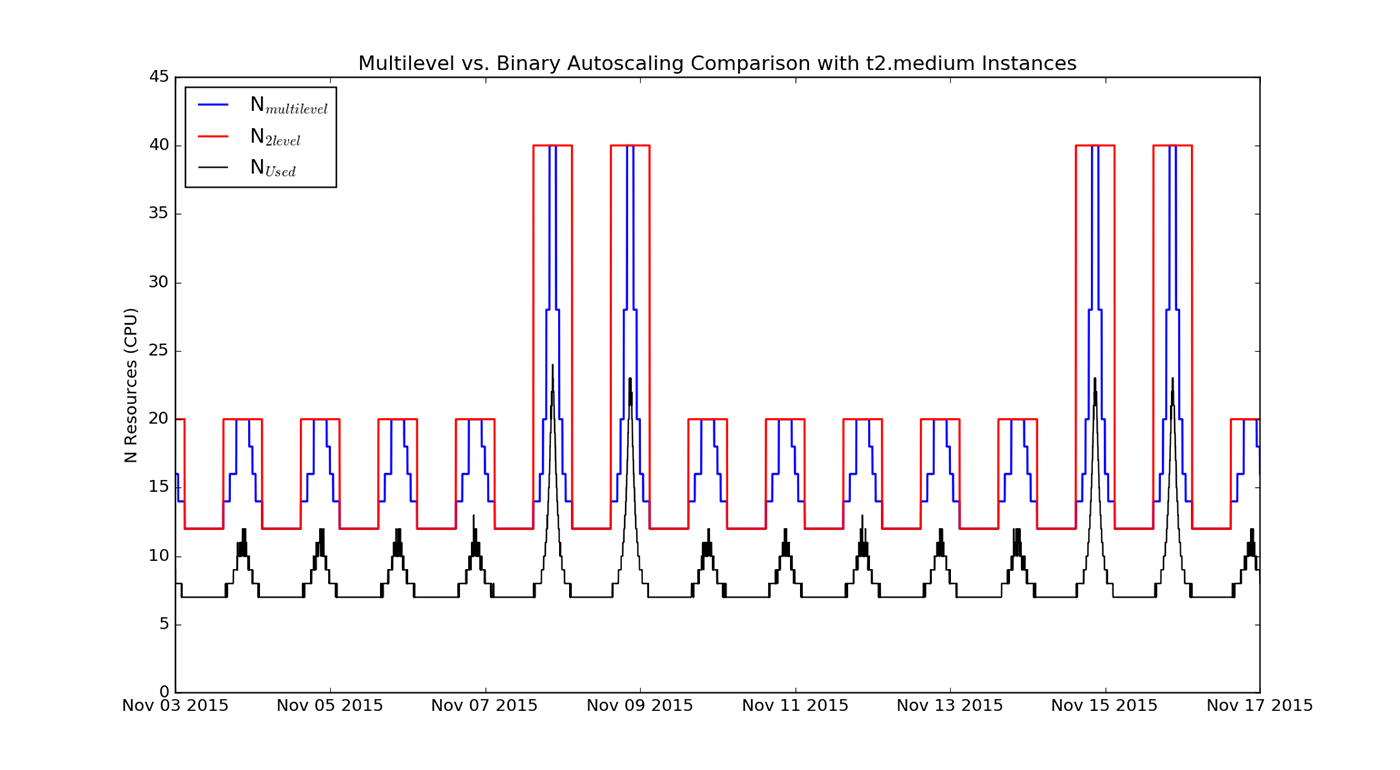
Figure 3 (below) illustrates how this setting would be implemented. The red line shows the binary schedule, including the difference between the weekday and weekend schedules. The blue line shows a more granular, multi-level schedule. The black line shows the actual usage:

It may be tempting to create even more detailed schedules, perhaps one for each day of the week, but we emphasize caution before proceeding. As discussed above, these analyses are based on only two weeks of usage data, and we lack sufficient information to assess whether these patterns are unique to this particular time of year. However, if we can determine that the observed pattern is consistent with what might be expected from the company’s business model, we can feel more confident in basing resource decisions upon it. The table below summarizes weekly cost estimates for a variety of schedules and instance types. It also includes pricing using dynamic Auto Scaling, which we’ll explore next.

Dynamic Auto Scaling

As we can see, using AWS’ Auto Scaling feature to schedule resources can lead to significant savings. At the same time, by using a multi-level schedule that hews closely to the observed usage pattern, a business also runs the risk that out-of-normal traffic can exceed the scheduled capacity. To avoid this, AWS offers a dynamic Auto Scaling capability that automatically adds or subtracts resources based upon pre-defined rules. For this usage pattern, we will consider a single scaling rule, though we note that AWS allows for multiple rules.

Let’s consider a rule where at any given time, if the usage exceeds 70% of available capacity, AWS should add 10% of the existing capacity. As usage falls off, AWS should subtract 20% of existing capacity when current usage falls below 55%. When setting this scaling rule, we must also account for the finite amount of time needed for a new instance to “warm up” before becoming operational.

For this scenario, we use AWS’s default setting of five minutes. Using this rule, we can step through our historical usage data to determine how many instances would be in use, launched, or deleted at any given time. Based on that output, we find that the average weekly cost for the period would be about $82, similar to the multi-level weekend + weekday schedule. This is not surprising when looking at historical data; our multi-level approach, which is optimized to the actual usage pattern, should produce similar results as dynamic, rules-based scaling.

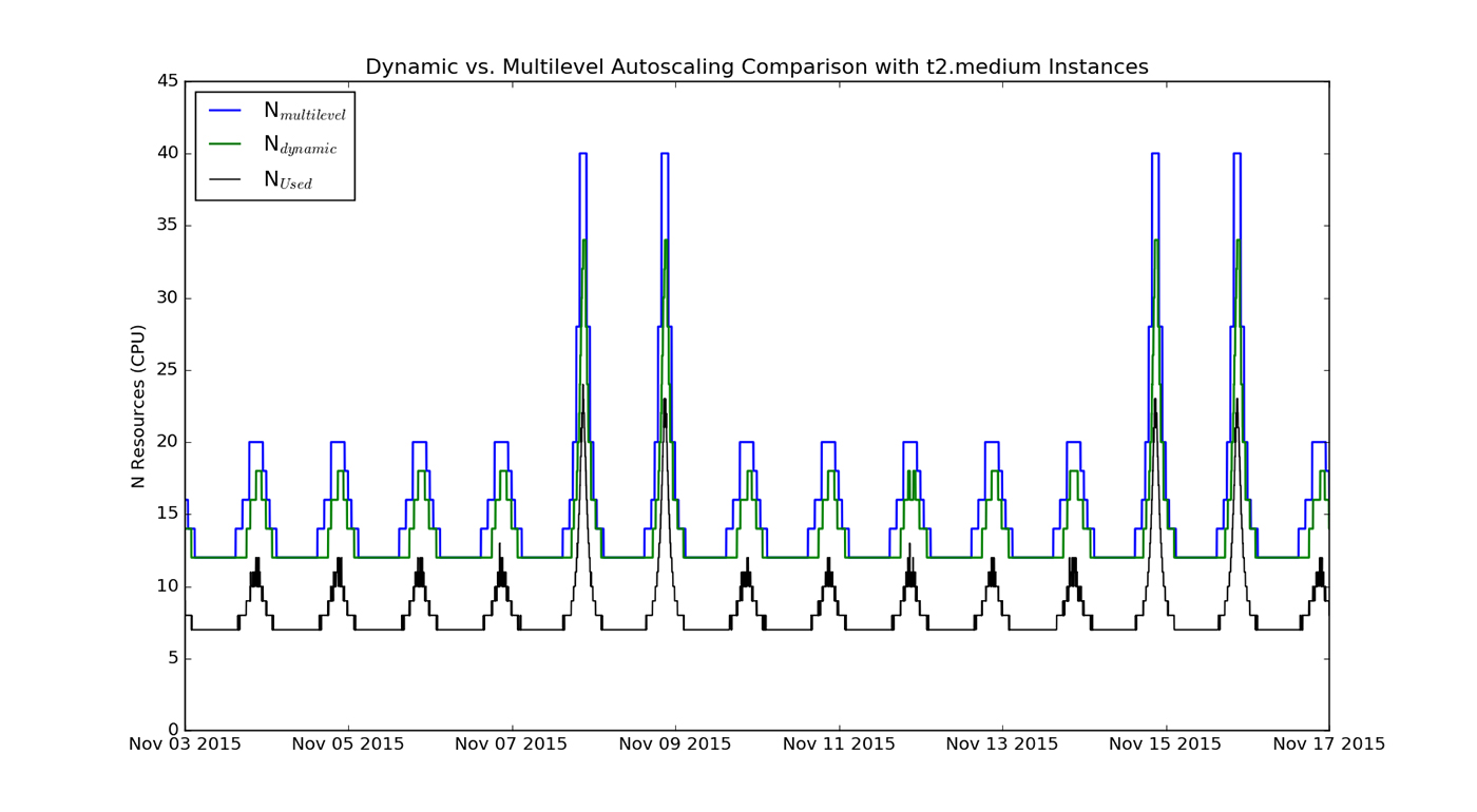
This can be seen in Figure 4, which shows the number of CPUs that would be made available from a multi-level schedule (blue line) and from dynamic Auto Scaling (green line). Notably, the highest resource level launched by dynamic Auto Scaling is lower than what is made available by the multi-level schedule, but the cost impact is not significant since the peak lasts for only a short duration. The main advantage of dynamic Auto Scaling compared to the multi-level schedule is that resources will still be added as needed even if the usage patterns deviate from historical behavior. For this usage pattern, this single rule is sufficient to provide substantial savings, though the optimal dynamic Auto Scaling setting will vary by each application’s web traffic. For more complex usage patterns, we could consider and analyze a more complex sets of rules:

Assess cost savings first

Third-party hosted, cloud-based infrastructure can offer businesses unprecedented advantages over private, on-site infrastructure. Cloud-based infrastructure can be deployed very quickly—saving months of procurement and set-up time. The use of dynamic resource scheduling, such as the capability enabled by AWS’s Auto Scaling tool, can also help significantly reduce costs by right-sizing infrastructure. As we have seen, however, determining the optimal settings for realizing the most savings requires detailed analyses of historical infrastructure usage patterns. Since re-engineering is often required to make applications work with changing numbers of resources, it is important businesses assess potential cost-savings prior to implementing Auto Scaling.

Note: This example was put together by Datapipe’s Data and Analytics Team.