Applying the Kappa architecture in the telco industry

Ever-growing volumes of data, shorter time constraints, and an increasing need for accuracy are defining the new analytics environment. In the telecom industry, traditional user and network data co­exists with machine-­to-­machine (M2M) traffic, media data, social activities, and so on. In terms of volume, this can be referred to as an “explosion” of data. This is a great business opportunity for telco operators and a key angle to take full advantage of current infrastructure investments (4G, LTE).

In this blog post, we will describe an approach to quickly ingest and analyze large volumes of streaming data, the Kappa architecture, as well as how to build a Bayesian online-­learning model to detect novelties in a complex environment. Note that novelty does not necessarily imply an undesired situation;  it indicates a change from previously known behaviours.

We apply both Kappa and the Bayesian model to a use case using a data stream originating from a telco cloud monitoring system. The stream is composed of telemetry and log events. It is high­ volume, as many physical servers and virtual machines are monitored simultaneously.

The proposed method quickly detects anomalies with high accuracy while adapting (learning) over time to new system normals, making it a desirable tool for considerably reducing maintenance costs associated with operability of large computing infrastructures.

What is “Kappa architecture”?

In a 2014 blog post, Jay Kreps accurately coined the term Kappa architecture by pointing out the pitfalls of the Lambda architecture and proposing a potential software evolution. To understand the differences between the two, let’s first observe what the Lambda architecture looks like:

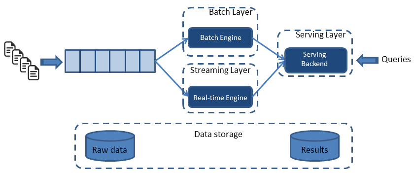
As shown in Figure 1, the Lambda architecture is composed of three layers: a batch layer, a real­-time (or streaming) layer, and a serving layer. Both the batch and real­-time layers receive a copy of the event, in parallel. The serving layer then aggregates and merges computation results from both layers into a complete answer.

The batch layer (aka, historical layer) has two major tasks: managing historical data and re­computing results such as machine learning models. Computations are based on iterating over the entire historical data set. Since the data set can be large, this produces accurate results at the cost of high latency due to high computation time.

The real­-time layer( speed layer, streaming layer) provides low-­latency results in near real-­time fashion. It performs updates using incremental algorithms, thus significantly reducing computation costs, often at the expense of accuracy.

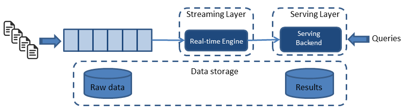
The Kappa architecture simplifies the Lambda architecture by removing the batch layer and replacing it with a streaming layer. To understand how this is possible, one must first understand that a batch is a data set with a start and an end (bounded), while a stream has no start or end and is infinite (unbounded). Because a batch is a bounded stream, one can conclude that batch processing is a subset of stream processing.  Hence, the Lambda batch layer results can also be obtained by using a streaming engine. This simplification reduces the architecture to a single streaming engine capable of ingesting the needed volumes of data to handle both batch and real-time processing. Overall system complexity significantly decreases with Kappa architecture. See Figure 2:

Intrinsically, there are four main principles in the Kappa architecture:

1. Everything is a stream: Batch operations become a subset of streaming operations. Hence, everything can be treated as a stream.
2. Immutable data sources: Raw data (data source) is persisted and views are derived, but a state can always be recomputed as the initial record is never changed.
3. Single analytics framework: Keep it short and simple (KISS) principle. A single analytics engine is required. Code, maintenance, and upgrades are considerably reduced.
4. Replay functionality: Computations and results can evolve by replaying the historical data from a stream.

In order to respect principle four, the data pipeline must guarantee that events stay in order from generation to ingestion. This is critical to guarantee consistency of results, as this guarantees deterministic computation results. Running the same data twice through a computation must produce the same result.

These four principles do, however, put constraints on building the analytics pipeline.

Building the analytics pipeline

Let ́s start concretizing how we can build such a data pipeline and identify the sorts of components required.

The first component is a scalable, distributed messaging system with events ordering and at-least-once delivery guarantees. Kafka can connect the output of one process to the input of another via a publish­-subscribe mechanism. Using it, we can build something similar to the Unix pipe systems where the output produced by one command is the input to the next.

The second component is a scalable stream analytics engine. Inspired by the Google Dataflow paper, Flink, at its core, is a streaming dataflow engine that provides data distribution, communication, and fault tolerance for distributed computations over data streams. One of its most interesting API features allows usage of the event timestamp to build time windows for computations.

The third and fourth components are a real-­time analytics store, Elasticsearch, and a powerful visualisation tool, Kibana. Those two components are not critical, but they’re useful to store and display raw data and results.

Mapping the Kappa architecture to its implementation, Figure 3 illustrates the resulting data pipeline:

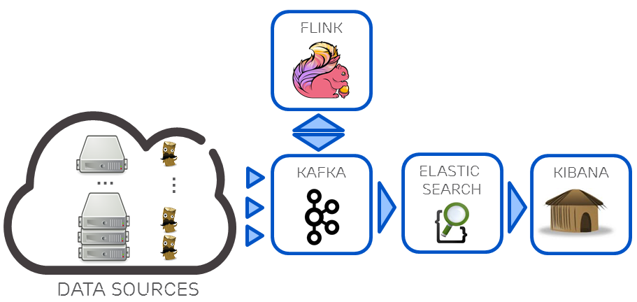
This pipeline creates a composable environment where outputs of different jobs can be re­used as inputs to another. Each job can thus be reduced to a simple, well-defined role. The composability allows for fast development of new features. In addition, data ordering and delivery are guaranteed, making results consistent. Finally, event timestamps can be used to build time windows for computations.

Applying the above to our telco use case, each physical host and virtual machine (VM) telemetry and log event is collected and sent to Kafka. We use collectd on the hosts, and ceilometer on the VMs for telemetry, and logstash-forwarder for logs. Kafka then delivers this data to different Flink jobs that transform and process the data. This monitoring gives us both the physical and virtual resource views of the system.

With the data pipeline in place, let’s look at how a Bayesian model can be used to detect novelties in a telco cloud.

Incorporating a Bayesian model to do advanced analytics

To detect novelties, we use a Bayesian model. In this context, novelties are defined as unpredicted situations that differ from previous observations. The main idea behind Bayesian statistics is to compare statistical distributions and determine how similar or different they are. The goal here is to:

• determine the distribution of parameters to detect an anomaly,
• compare new samples for each parameter against calculated distributions and determine if the obtained value is expected or not,
• and combine all parameters to determine if there is an anomaly.

Let’s dive into the math to explain how we can perform this operation in our analytics framework. Considering the anomaly A, a new sample z, θ observed parameters, P(θ) the probability distribution of the parameter, A(z|θ) the probability that z is an anomaly, X the samples, the Bayesian Principal Anomaly can be written as:

A (z | X) = ∫A(θ)P(θ|X)

A principal anomaly as defined above is valid also for multi­variate distributions. The approach taken evaluates the anomaly for each variable separately, and then combines them into a total anomaly value.

An anomaly detector considers only a small part of the variables, and typically only a single variable with a simple distribution like Poisson or Gauss, can be called a micro­model. A micromodel with gaussian distribution will look like this:

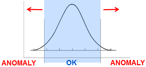
An array of micro­models can then be formed, with one micro­model per variable (or small set of variables). Such an array can be called a component. The anomaly values from the individual detectors then have to be combined into one anomaly value for the whole component. The combination depends on the use case. Since accuracy is important (avoid false positives) and parameters can be assumed to be fairly independent from one another, then the principal anomaly for the component can be calculated as the maximum of the micro­model anomalies, but scaled down to meet the correct false alarm rate (i.e., weighted influence of components to improve the accuracy of the principal anomaly detection).

However, there may be many different “normal” situations. For example, the normal system behavior may vary within weekdays or time of day. Then, it may be necessary to model this with several components, where each component learns the distribution of one cluster. When a new sample arrives, it is tested by each component. If it is considered anomalous by all components, it is considered as anomalous. If any component finds the sample normal, then it is normal.

Applying this to our use case, we used this detector to spot errors or deviations from normal operations in a telco cloud. Each parameter θ is any of the captured metrics or logs resulting in many micromodels. By keeping a history of past models, and computing a principal anomaly for the component, we can find statistically relevant novelties. These novelties could come from configuration errors, a new error in the infrastructure, or simply a new state of the overall system (i.e., a new set of virtual machines).

Using the number of generated logs (or log frequency) appears to be the most significant feature to detect novelties. By modeling the statistical function of generated logs over time (or log frequency), the model can spot errors or novelties accurately. For example, let’s consider the case where a database becomes unavailable. At that time, any applications depending on it start logging recurring errors, (e.g., “Database X is unreachable…”). This raises the log frequency, which triggers a novelty in our model and detector.

The overall data pipeline, combining the transformations mentioned before, will look like this:

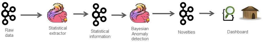
This data pipeline receives the raw data, extracts statistical information (such as log frequencies per machine), applies the Bayesian anomaly detector over the interesting features (statistical and raw), and outputs novelties whenever they are found.

Conclusion

In this blog post, we have presented an approach using the Kappa architecture and a self-training (online) Bayesian model to yield quick, accurate analytics.

The Kappa architecture allows us to develop a new generation of analytics systems. Remember, this architecture has four main principles: data is immutable, everything is a steam, a single stream engine is used, and data can be replayed. It simplifies both the software systems and the development and maintenance of machine learning models. Those principles can easily be applied to most use cases.

The Bayesian model quickly detects novelties in our cloud. This type of online learning has the advantage of adapting over time to new situations, but one of its main challenges is a lack of ready­-to-­use algorithms. However, the analytics landscape is evolving fast and we are confident that a richer environment can be expected in the near future.

Ignacio Mulas Viela and Nicolas Seyvet will speak in greater detail on this topic as well as on a telco data set from a running cloud during their session Kappa architecture in the telecom industry at Strata + Hadoop World London 2016, May 31 to June 3, 2016.