 Neurons. (source: Pixabay)
 Chainer is an open source framework designed for efficient research into and development of deep learning algorithms. In this post, we briefly introduce Chainer with a few examples and compare with other frameworks such as Caffe, Theano, Torch, and Tensorflow.
Most existing frameworks construct a computational graph in advance of training. This approach is fairly straightforward, especially for implementing fixed and layer-wise neural networks like convolutional neural networks.
However, state-of-the-art performance and new applications are now coming from more complex networks, such as recurrent or stochastic neural networks. Though existing frameworks can be used for these kinds of complex networks, it sometimes requires (dirty) hacks that can reduce development efficiency and maintainability of the code.
Chainer’s approach is unique: building the computational graph “on-the-fly” during training.
This allows users to change the graph at each iteration or for each sample, depending on conditions. It is also easy to debug and refactor Chainer-based code with a standard debugger and profiler, since Chainer provides an imperative API in plain Python and NumPy. This gives much greater flexibility in the implementation of complex neural networks, which leads in turn to faster iteration, and greater ability to quickly realize cutting-edge deep learning algorithms.
Below, I describe how Chainer actually works and what kind of benefits users can get from it.
Chainer basics
Chainer is a standalone deep learning framework based on Python.
Unlike other frameworks with a Python interface such as Theano and TensorFlow, Chainer provides imperative ways of declaring neural networks by supporting Numpy-compatible operations between arrays. Chainer also includes a GPU-based numerical computation library named CuPy.
>>> from chainer import Variable
>>> import numpy as np
A class Variable represents the unit of computation by wrapping numpy.ndarray in it (.data).
>>> x = Variable(np.asarray([[0, 2],[1, -3]]).astype(np.float32))
>>> print(x.data)
[[ 0.      2.]
 [ 1.     -3.]]
Users can define operations and functions (instances of Function) directly on Variables.
>>> y = x ** 2 - x + 1
>>> print(y.data)
[[  1.   3.]
 [  1.  13.]]
Since Variables remember what they are generated from, Variable y has the additive operation as its parent (.creator).
>>> print(y.creator)
<chainer.functions.math.basic_math.AddConstant at 0x7f939XXXXX>
This mechanism makes backword computation possible by tracking back the entire path from the final loss function to the input, which is memorized through the execution of forward computation—without defining the computational graph in advance.
Many numerical operations and activation functions are given in chainer.functions. Standard neural network operations such as fully connected linear and convolutional layers are implemented in Chainer as an instance of Link. A Link can be thought of as a function together with its corresponding learnable parameters (such as weight and bias parameters, for example). It is also possible to create a Link that itself contains several other links. Such a container of links is called a Chain. This allows Chainer to support modeling a neural network as a hierarchy of links and chains. Chainer also supports state-of-the-art optimization methods, serialization, and CUDA-powered faster computations with CuPy.
>>> import chainer.functions as F
>>> import chainer.links as L
>>> from chainer import Chain, optimizers, serializers, cuda
>>> import cupy as cp
Chainer’s design: Define-by-Run
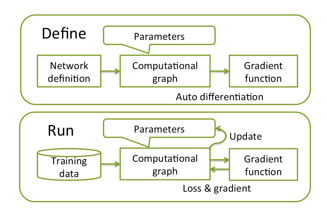
To train a neural network, three steps are needed: (1) build a computational graph from network definition, (2) input training data and compute the loss function, and (3) update the parameters using an optimizer and repeat until convergence.
Usually, DL frameworks complete step one in advance of step two. We call this approach define-and-run.
This is straightforward but not optimal for complex neural networks since the graph must be fixed before training. Therefore, when implementing recurrent neural networks, for examples, users are forced to exploit special tricks (such as the scan() function in Theano) which make it harder to debug and maintain the code.
Instead, Chainer uses a unique approach called define-by-run, which combines steps one and two into a single step.

The computational graph is not given before training but obtained in the course of training. Since forward computation directly corresponds to the computational graph and backpropagation through it, any modifications to the computational graph can be done in the forward computation at each iteration and even for each sample.
As a simple example, let’s see what happens using two-layer perceptron for MNIST digit classification.
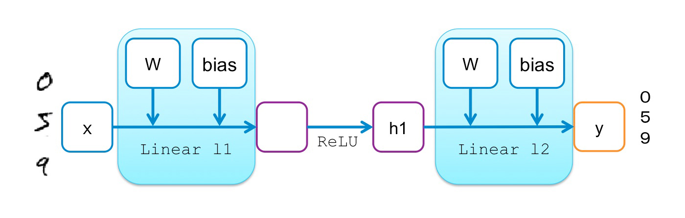
The following code shows the implementation of two-layer perceptron in Chainer:
# 2-layer Multi-Layer Perceptron (MLP)
class MLP(Chain):

    def __init__(self):
        super(MLP, self).__init__(
            l1=L.Linear(784, 100),  # From 784-dimensional input to hidden unit with 100 nodes
            l2=L.Linear(100, 10),  # From hidden unit with 100 nodes to output unit with 10 nodes  (10 classes)
        )

    # Forward computation
    def __call__(self, x):
        h1 = F.tanh(self.l1(x))     # Forward from x to h1 through activation with tanh function
        y = self.l2(h1)                 # Forward from h1to y
			        return y
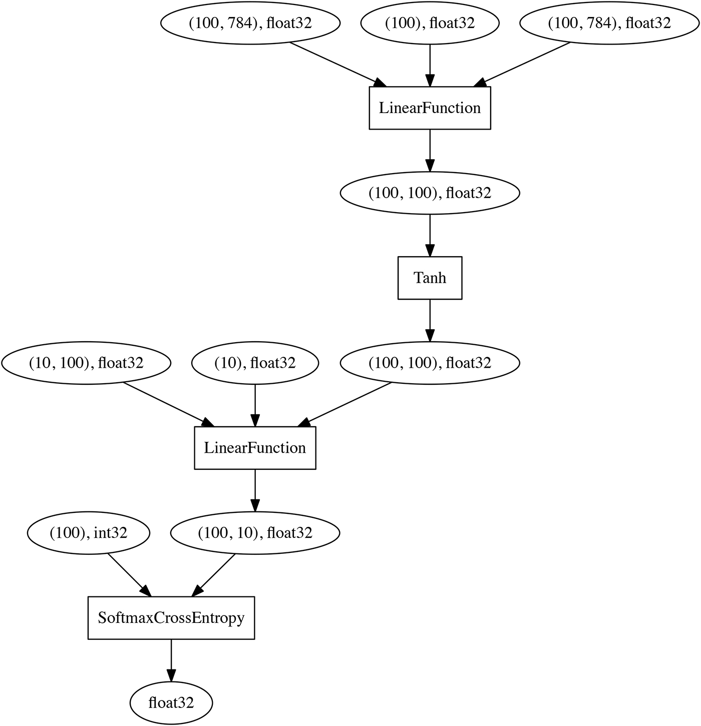
In the constructer (__init__), we define two linear transformations from the input to hidden units, and hidden to output units, respectively. Note that no connection between these transformations is defined at this point, which means that the computation graph is not even generated, let alone fixed.
Instead, their relationship will be later given in the forward computation (__call__), by defining the activation function (F.tanh) between the layers. Once forward computation is finished for a minibatch on the MNIST training data set (784 dimensions), the following computational graph can be obtained on-the-fly by backtracking from the final node (the output of the loss function) to the input (note that SoftmaxCrossEntropy is also introduced as the loss function):
The point is that the network definition is simply represented in Python rather than a domain-specific language, so users can make changes to the network in each iteration (forward computation).
This imperative declaration of neural networks allows users to use standard Python syntax for branching, without studying any domain specific language (DSL), which can be beneficial as compared to the symbolic approaches that TensorFlow and Theano utilize and also the text DSL that Caffe and CNTK rely on.
In addition, a standard debugger and profiler can be used to find the bugs, refactor the code, and also tune the hyper-parameters. On the other hand, although Torch and MXNet also allow users to employ imperative modeling of neural networks, they still use the define-and-run approach for building a computational graph object, so debugging requires special care.
Implementing complex neural networks
The above is just an example of a simple and fixed neural network. Next, let’s look at how complex neural networks can be implemented in Chainer.
A recurrent neural network is a type of neural network that takes sequence as input, so it is frequently used for tasks in natural language processing such as sequence-to-sequence translation and question answering systems. It updates the internal state depending not only on each tuple from the input sequence, but also on its previous state so it can take into account dependencies across the sequence of tuples.
Since the computational graph of a recurrent neural network contains directed edges between previous and current time steps, its construction and backpropagation are different from those for fixed neural networks, such as convolutional neural networks. In current practice, such cyclic computational graphs are unfolded into a directed acyclic graph each time for model update by a method called truncated backpropagation through time.
For this example, the target task is to predict the next word given a part of sentence. A successfully trained neural network is expected to generate syntactically correct words rather than random words, even if the entire sentence does not make sense to humans. The following example shows a simple recurrent neural network with one recurrent hidden unit:
# Definition of simple recurrent neural network
class SimpleRNN(Chain):

    def __init__(self, n_vocab, n_nodes):
        super(SimpleRNN, self).__init__(
            embed=L.EmbedID(n_vocab, n_nodes),  # word embedding
            x2h=L.Linear(n_nodes, n_nodes),  # the first linear layer
            h2h=L.Linear(n_nodes, n_nodes),  # the second linear layer
            h2y=L.Linear(n_nodes, n_vocab),  # the feed-forward output layer
        )
        self.h_internal=None # recurrent state

    def forward_one_step(self, x, h):
        x = F.tanh(self.embed(x))
        if h is None: # branching in network
            h = F.tanh(self.x2h(x))
        else:
            h = F.tanh(self.x2h(x) + self.h2h(h))
        y = self.h2y(h)
        return y, h

    def __call__(self, x):
        # given the current word ID, predict the next word ID.
        y, h = self.forward_one_step(x, self.h_internal)
        self.h_internal = h # update internal state
        return y
Only the types and size of layers are defined in the constructor as well as on the multi-layer perceptron. Given input word and current state as arguments, forward_one_step() method returns output word and new state. In the forward computation (__call__), forward_one_step() is called for each step and updates the hidden recurrent state with a new one.
By using the popular text data set Penn Treebank (PTB), we trained a model to predict the next word from probable vocabularies. Then the trained model is used to predict subsequent words using weighted sampling.
"If you build it," => "would a outlawed a out a tumor a colonial a"
"If you build it, they" => " a passed a president a glad a senate a billion"
"If you build it, they will" => " for a billing a jerome a contracting a surgical a"
"If you build it, they will come" => "a interviewed a invites a boren a illustrated a pinnacle"
This model has learned—and then produced—many repeated pairs of “a” and a noun or an adjective. Which means “a” is one of the most probable words, and a noun or adjective tend to follow after “a.”
To humans, the results look almost the same, being syntactically wrong and meaningless, even when using different inputs. However, these are definitely inferred based on the real sentences in the data set by training the type of words and relationship between them.
Though this is inevitable due to the lack of expressiveness in the SimpleRNN model, the point here is that users can implement any kinds of recurrent neural networks just like SimpleRNN.
Just for comparison, by using off-the-shelf mode of recurrent neural network called Long Short Term Memory (LSTM), the generated texts become more syntactically correct.
"If you build it," => "pension say computer ira <EOS> a week ago the japanese"
"If you buildt it, they" => "were jointly expecting but too well put the <unknown> to"
"If you build it, they will" => "see the <unknown> level that would arrive in a relevant"
"If you build it, they will come" => "to teachers without an mess <EOS> but he says store"
Since popular RNN components such as LSTM and gated recurrent unit (GRU) have already been implemented in most of the frameworks, users do not need to care about the underlying implementations. However, if you want to significantly modify them or make a completely new algorithm and components, the flexibility of Chainer makes a great difference compared to other frameworks.
Stochastically changing neural networks
In the same way, it is very easy to implement stochastically changing neural networks with Chainer.
The following is mock code to implement Stochastic ResNet. In __call__, just flip a skewed coin with probability p, and change the forward path by having or not having unit f. This is done at each iteration for each minibatch, and the memorized computational graph is different each time but updated accordingly with backpropagation after computing the loss function.
# Mock code of Stochastic ResNet in Chainer
class StochasticResNet(Chain):

  def __init__(self, prob, size, **kwargs):
    super(StochasticResNet, self).__init__(size, **kwargs)
    self.p = prob # Survival probabilities

  def __call__ (self, h):
    for i in range(self.size):
      b = numpy.random.binomial(1, self.p[i])
      c = self.f[i](h) + h if b == 1 else h
      h = F.relu(c)
    return h
Conclusion
In addition to the above, Chainer has many features to help users to realize neural networks for their tasks as easily and efficiently as possible.
CuPy is a NumPy-equivalent array backend for GPUs included in Chainer, which enables CPU/GPU-agnostic coding, just like NumPy-based operations. The training loop and data set handling can be abstracted by Trainer, which keeps users away from writing such routines every time, and allows them to focus on writing innovative algorithms. Though scalability and performance are not the main focus of Chainer, it is still competitive with other frameworks, as shown in the public benchmark results, by making full use of NVIDIA’s CUDA and cuDNN.
Chainer has been used in many academic papers not only for computer vision, but also speech processing, natural language processing, and robotics. Moreover, Chainer is gaining popularity in many industries since it is good for research and development of new products and services. Toyota motors, Panasonic, and FANUC are among the companies that use Chainer extensively and have shown some demonstrations, in partnership with the original Chainer developement team at Preferred Networks.
Interested readers are encouraged to visit the Chainer website for further details. I hope Chainer will make a difference for many cutting-edge research and real-world products based on deep learning!