A Signal Theoretic Introduction to Random Processes

7CHARACTERIZING RANDOM PROCESSES

7.1 INTRODUCTION

There are many ways a random process can be characterized, and the characterization is usually linked to the application or situation in which it arises and the information required. The most common ways of characterizing random processes is via the evolution with time of the probability mass/density function, an autocorrelation function, and a power spectral density function. This chapter provides an introduction to such characterization, and this is followed by associated material including correlation, the average power in a random process, stationarity, Cramer’s representation of random processes, and the state space characterization of random processes. One-dimensional random processes are assumed.

7.1.1 Notation for One-Dimensional Random Processes

Consistent with the notation introduced in Chapter 5 and used in Chapter 6, the following notation is used for a random process X:

(7.1)

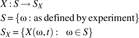
For notational convenience, a random process is written as X(Ω, t) with the interpretation

(7.2)

The probability of a specific experimental outcome is governed by a probability mass function or a probability density function:

(7.3)

In this chapter, the signals are assumed to be one-dimensional as illustrated in Figure 7.1.

Figure ...