A Workout in Computational Finance

8 Solving Systems of Linear Equations

As pointed out in the previous chapters, the discretization of partial differential equations with finite difference or finite element methods in connection with implicit or semi-implicit time-stepping schemes results in large systems of linear equations,

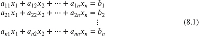
or, in matrix-vector form,

The matrix A is called the coefficient matrix, x is the vector of unknowns and b the right-hand side. We will restrict ourselves to systems with quadratic coefficient matrices:¹ for a number of n unknowns (the length of the vector x), the dimension of A is n × n. Furthermore, we will assume that the coefficient matrix is regular (rank of A = n).

Depending on the financial model chosen and the desired accuracy of the discretization scheme, the sparsity of the coefficient matrix A can range from tridiagonal² to dense.³ There are many different algorithms available for solving linear systems. In order to choose the optimal algorithm for a given problem, a number of factors must be considered:

• System size: for large n, direct methods become inefficient in terms of speed and memory usage, and iterative solvers should be preferred.
• Sparsity: if the number of zero matrix entries a_ij = 0 in the matrix is large (which is typically the case in banded matrices), methods where ...