Adjustment Computations, 6th Edition

APPENDIX CNONLINEAR EQUATIONS AND TAYLOR'S THEOREM

C.1 INTRODUCTION

In adjustment computations, it is frequently necessary to deal with nonlinear equations. For example, some observation equations relate observed quantities to unknown parameters through the transcendental functions of sine, cosine, or tangent, while others relate them through terms raised to second- and higher-order powers. The task of solving a system of nonlinear equations is formidable. To facilitate the solution, a first-order Taylor series approximation can be used to create a set of linear equations. The equations can then be solved by matrix methods discussed in Appendix A.

C.2 TAYLOR SERIES LINEARIZATION OF NONLINEAR EQUATIONS

Suppose that the following equation relates an observed value L to its unknown parameters x and y through nonlinear coefficients as

(C.1)

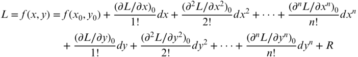
By Taylor's theorem, the equation can be represented as

(C.2)

In Equation (C.2), x₀ and y₀ are approximations for x and y; f(x₀, y₀) is the nonlinear function evaluated at these approximations; R is the remainder, and dx and dy are corrections to the approximations, such that

(C.3)

A more exact Taylor series approximation is obtained by ...